

The BITXOR function in Excel looks at two numbers in binary, one bit at a time, and gives you back a number with a 1 wherever the two don’t match. It’s the bitwise version of the XOR function, which works with TRUE and FALSE.
That “keep what’s different” behavior is handy when one number stores several yes/no options. You can use it to spot what changed between two codes, flip a single option on or off, or hide a number behind a secret key and get it back later.
I’ll show you six examples below, starting with two plain numbers and ending with a set of locker PINs.
Follow along with the example file
BITXOR Function Examples.xlsx
BITXOR Function Syntax
Here is the syntax of the BITXOR function:
=BITXOR(number1, number2)
- number1 – The first number. It must be a whole number that is 0 or more.
- number2 – The second number, with the same rules as number1.
BITXOR turns both numbers into binary and compares them one position at a time. It puts a 1 where only one of the numbers has a 1, and a 0 where both numbers match, and then gives you the result as a regular decimal number.
Both numbers must be between 0 and 281,474,976,710,655 (that’s 2^48-1). A negative number or anything larger returns the #NUM! error.
BITXOR also doesn’t round or cut off decimals. A number like 13.9 returns #NUM!, so if your numbers come from a calculation, wrap them in the INT or ROUND function first.
Numbers stored as text, like “12”, work fine, and an empty cell counts as 0. Text that isn’t a number, like “abc”, returns the #VALUE! error.
The BITXOR function works in Excel 2013 and later versions, including Microsoft 365, Excel 2024, 2021, 2019, 2016, and Excel for Mac.
When to Use the BITXOR Function
Use this function when you need to:
- Compare two numbers bit by bit and keep only the bits where they differ
- Flip one option in a code, turning it off if it’s on and on if it’s off
- Find which options changed between an old code and a new code
- Count how many options are different between two codes
- Hide a number with a secret key and get the original back later
Let me show you a few practical examples of how to use the BITXOR function.
Example 1: Use BITXOR to Compare Two Numbers
Let’s start with a simple example so you can see what BITXOR does with plain numbers.
Below I have some pairs of numbers, and I want to get the BITXOR result of each pair in column C.
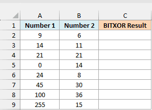
Here is the formula:
=BITXOR(A2:A9,B2:B9)
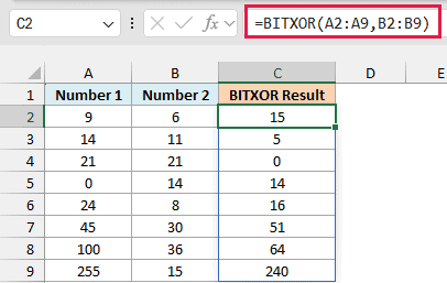
Enter this in cell C2, and it spills the results down to C9. BITXOR goes row by row and compares the number in column A with the number in column B.
To see where the 5 for 14 and 11 (in row 3) comes from, here are both numbers written in binary, with the value of each position at the top:
| Number | 8 | 4 | 2 | 1 |
|---|---|---|---|---|
| 14 | 1 | 1 | 1 | 0 |
| 11 | 1 | 0 | 1 | 1 |
| BITXOR result | 0 | 1 | 0 | 1 |
The two numbers are different only in the 4 and 1 positions, so BITXOR returns 4 + 1 = 5. The 8 and 2 positions have a 1 in both numbers, so they drop out.
That’s also why 21 and 21 return 0. When both numbers are the same, there’s no position where they differ.
And when one of the numbers is 0, like 0 and 14, you simply get the other number back.
If you are using Excel 2019 or earlier, enter the below formula in cell C2 and then copy it down the range:
=BITXOR(A2,B2)
Example 2: Flip One Option in a Code
Now let’s look at where BITXOR gets really useful.
Below is a list of app users with a code for their notification settings, and I want to flip the Weekly Digest setting for each user and get the new code in column C.
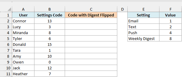
The table on the right shows the value of each setting. A user’s code is the total of the settings they have turned on, so Connor’s code of 13 means Email (1), Push (4), and Weekly Digest (8).
Here is the formula:
=BITXOR(B2:B11,F5)
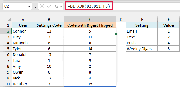
The setting values 1, 2, 4, and 8 are the same binary positions you saw in Example 1, so each setting is its own bit in the code.
Cell F5 holds 8, the value of Weekly Digest. BITXOR flips only the 8 bit in each code and leaves every other setting as it is.
So Connor had Weekly Digest on, and his code drops from 13 to 5. Lucy had it off, and her code goes from 3 to 11.
Important: BITXOR switches the setting off for anyone who already has it on. If you want to turn a setting on for everyone, no matter what it was before, use the BITOR function instead.
Since it’s a flip, running BITXOR with 8 again on the new codes takes everyone back to their original settings. To flip a different setting, point the formula to its value instead, like F2 for Email.
If you are using Excel 2019 or earlier, enter the below formula in cell C2 and then copy it down the range:
=BITXOR(B2,$F$5)
Example 3: Find Which Options Changed Between Two Codes
Here’s another practical scenario.
Below is a list of streaming subscribers with their add-ons code for last month and this month, and I want to find which add-ons changed in column D.
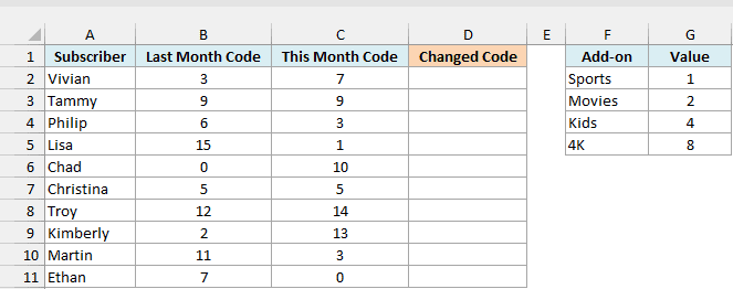
The table on the right shows the value of each add-on, with Sports as 1, Movies as 2, Kids as 4, and 4K as 8.
Here is the formula:
=BITXOR(B2:B11,C2:C11)
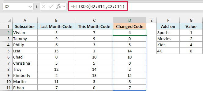
The result is a code made up of every add-on that is in one month but not the other. Vivian went from 3 (Sports, Movies) to 7 (Sports, Movies, Kids), so her changed code is 4, which is Kids.
Lisa went from 15 to 1, so her changed code is 14, which is Movies, Kids, and 4K. Tammy and Christina get 0 because their add-ons didn’t change at all.
Note that BITXOR doesn’t tell you whether an add-on was added or dropped. Philip’s changed code of 5 is Sports and Kids, and you can see that Sports is in this month’s code (3) while Kids isn’t, so he added Sports and dropped Kids.
You can also get Excel to do that split with the BITAND function, which keeps only the bits two numbers share. For Philip, using it on his changed code (5) and this month’s code (3) returns 1, which is Sports, the add-on he added.
Do the same with last month’s code (6), and you get 4, which is Kids, the add-on he dropped.
If you are using Excel 2019 or earlier, enter the below formula in cell D2 and then copy it down the range:
=BITXOR(B2,C2)
Example 4: Count How Many Options Changed
A changed code like 14 doesn’t tell you at a glance how many add-ons changed, so let’s count them.
Using the same streaming subscribers, I now want to get the number of add-ons that changed for each subscriber in column E.
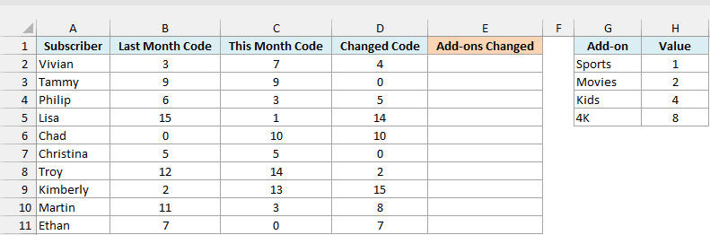
Here is the formula:
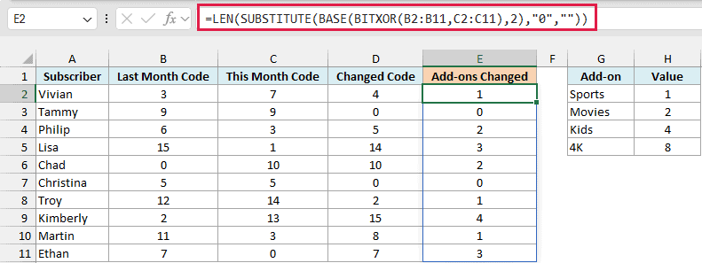
=LEN(SUBSTITUTE(BASE(BITXOR(B2:B11,C2:C11),2),"0",""))
How this formula works:
- BITXOR(B2:B11,C2:C11) gets the changed code for each subscriber, just like in Example 3.
- The BASE function, with 2 as the base, turns each changed code into binary text. For example, Lisa’s 14 becomes “1110”.
- The SUBSTITUTE function removes all the 0s, so “1110” becomes “111”.
- The LEN function counts the characters that are left, which is the number of 1s, and every 1 is one changed add-on.
So Lisa gets 3, and Kimberly, who went from 2 to 13, gets 4 because every one of her add-ons changed. A changed code of 0 becomes “0” in binary, which turns into empty text, so Tammy and Christina get 0.
If you are using Excel 2019 or earlier, enter the below formula in cell E2 and then copy it down the range:
=LEN(SUBSTITUTE(BASE(BITXOR(B2,C2),2),"0",""))
Example 5: List the Options That Don’t Match
Let’s step it up with a more advanced use case, where BITXOR finds the mismatches and the result comes back as names instead of a code.
Below is a list of pizza orders with a code for the toppings each customer ordered and a code for the toppings that were delivered, and I want to list the toppings that don’t match in column D.
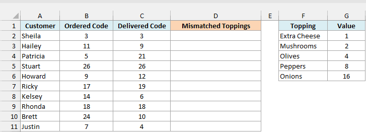
The table on the right shows the value of each topping, from 1 for Extra Cheese up to 16 for Onions.
Here is the formula:
=MAP(B2:B11,C2:C11,LAMBDA(ordered,delivered,TEXTJOIN(", ",TRUE,FILTER(F2:F6,BITAND(BITXOR(ordered,delivered),G2:G6),"All correct"))))
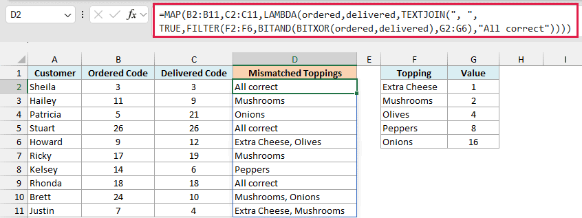
The earlier examples spilled by giving BITXOR whole ranges, but that doesn’t work here. The TEXTJOIN function joins everything it gets into one cell, so it would lump every order’s toppings together.
That’s why this formula uses the MAP function, which runs the calculation once for each order.
How this formula works:
- The MAP function goes through the orders one at a time and passes each ordered code and delivered code to the LAMBDA function as ordered and delivered.
- BITXOR(ordered,delivered) returns a code with every topping that’s in one code but not the other.
- The BITAND function checks that code against each topping value in G2:G6 and returns a number other than 0 for the toppings that don’t match.
- The FILTER function keeps those topping names, and returns “All correct” when nothing is wrong.
- The TEXTJOIN function combines the names into one text, separated by a comma and a space.
So Howard ordered 9 (Extra Cheese, Peppers) but got 12 (Olives, Peppers), and his result is “Extra Cheese, Olives”. The cheese is missing and the olives shouldn’t be there, but the Peppers match, so they don’t show up.
The MAP function works in Excel 365 and Excel 2024. If you are using Excel 2021, enter the below formula in cell D2 and then copy it down the range:
=TEXTJOIN(", ",TRUE,FILTER($F$2:$F$6,BITAND(BITXOR(B2,C2),$G$2:$G$6),"All correct"))
This example needs Excel 2021 or later, because the FILTER function isn’t available in Excel 2019 and earlier.
Example 6: Encode and Decode a Number with a Secret Key
Let’s end with a fun one that uses a special property of BITXOR. If you apply it twice with the same number, you get back exactly what you started with.
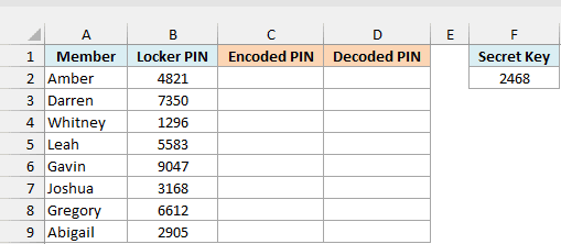
Below is a list of gym members with their locker PINs, and I want to hide each PIN in column C using the secret key in cell F2, and then get the original PIN back in column D.
Here is the formula that encodes the PINs:
=BITXOR(B2:B9,F2)
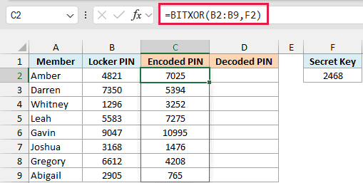
BITXOR flips every bit in each PIN where the key 2468 has a 1. So Amber’s PIN of 4821 becomes 7025, which looks nothing like the original.
The encoded number doesn’t always have four digits. Gavin’s 9047 becomes 10995, and Abigail’s 2905 becomes 765.
If you are using Excel 2019 or earlier, enter the below formula in cell C2 and then copy it down the range:
=BITXOR(B2,$F$2)
And here is the formula that decodes them:
=BITXOR(C2:C9,F2)
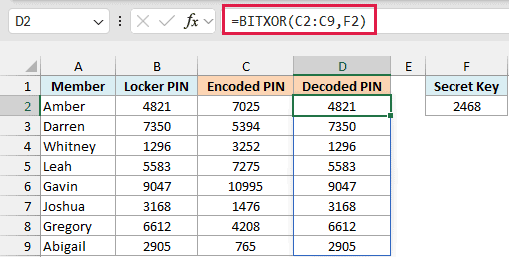
This applies the same key to the encoded PINs. Every bit the first formula flipped gets flipped back, so 7025 turns back into 4821, and every row in column D matches column B.
If you are using Excel 2019 or earlier, enter the below formula in cell D2 and then copy it down the range:
=BITXOR(C2,$F$2)
Keep in mind that this only stops someone from reading the PINs at a glance, and it is not real security. Anyone who has the key (or knows this trick) can decode them, so don’t use it to protect anything sensitive.
So these are some practical ways to use the BITXOR function in Excel. Whenever you need to know how two codes differ, or flip one option without touching the others, BITXOR does it in one step.
Just make sure both numbers are whole and not negative, or you’ll get the #NUM! error. I hope you found this article helpful.
Other Excel Articles You May Also Like:
