

The YIELDMAT function in Excel returns the annual yield of a security that pays all its interest in one lump sum at maturity. A common example is a CD (certificate of deposit) bought from another investor through a brokerage, after the bank first issued it.
The stated interest rate doesn’t tell you what you’ll earn on a CD like that.
You pay a market price (quoted per $100 of face value, so a little above or below 100), plus the interest built up since the issue date. YIELDMAT turns all of that into one annual percentage.
In this article, I start with a single CD and then a list of CDs. After that, I show how to rank them, how to work from a trade confirmation, how YIELDMAT calculates its result, and how to find the price for a target yield.
Follow along with the example file
YIELDMAT Function Examples.xlsx
YIELDMAT Function Syntax
Here is the syntax of the YIELDMAT function:
=YIELDMAT(settlement,maturity,issue,rate,pr,[basis])
- settlement – the date you buy the security (the date the trade settles, not the date it was first issued).
- maturity – the date the security matures and pays back its face value plus all its interest.
- issue – the date the security was first issued. Interest starts building up from this date.
- rate – the security’s annual interest rate, such as 4.25%.
- pr – the price you pay per $100 of face value, without the interest that has built up since the issue date.
- [basis] – optional. The day count method, which sets how Excel counts the days between dates: 0 (US 30/360, which treats every month as 30 days), 1 (actual/actual), 2 (actual/360), 3 (actual/365), or 4 (European 30/360). If you leave it out, Excel uses 0.
Notice that maturity comes before issue in the arguments, even though the issue date comes first on the calendar. If you swap the two, YIELDMAT returns the #NUM! error.
The dates also need to be in order: the issue date first, then the settlement date, then the maturity date. If the settlement date is on or before the issue date, or on or after the maturity date, you get the #NUM! error.
This means you can’t use YIELDMAT for a CD you buy on the day it’s issued. If you buy it at 100 on that day, its yield is exactly its interest rate.
For a short security, the basis barely moves the result. For the CD in Example 1, switching from 0 to 3 changes the yield by less than 0.001 percentage points, but still use the day count given in the security’s terms.
The dates should be real dates in cells, or dates built with the DATE function. If Excel can’t read a date, YIELDMAT returns the #VALUE! error.
The YIELDMAT function works in Excel 365, 2024, 2021, 2019, 2016, and Excel for Mac.
When to Use the YIELDMAT Function
Use this function when you need to:
- Find the yield of a CD or note that pays all its interest at maturity, when you buy it after its issue date
- Compare offers on several such CDs that have different rates, prices, and dates
- Check the return on a trade confirmation from your broker
- Work out the highest price you can pay to get a target yield
Let me show you a few practical examples of how to use the YIELDMAT function.
Example 1: Calculate the Yield of a CD in Excel
Let’s start with a single CD.
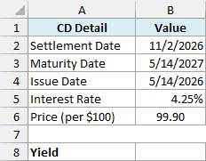
This 12-month CD was issued on May 14, 2026, pays 4.25% interest at maturity, and is being sold by another investor for 99.90 per $100.
Below are the details of the CD, and I want to get its yield in cell B8.
Here is the formula:
=YIELDMAT(B2,B3,B4,B5,B6)
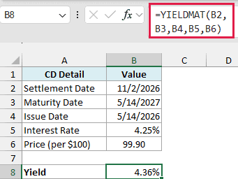
The formula returns 4.36%, which is a little higher than the CD’s 4.25% interest rate.
Two things affect this. You pay 99.90 and get back 100 at maturity, and that extra 0.10, earned in about six months, pushes the yield up.
You also pay the seller the interest built up since May 14, and that money earns you nothing, which pulls the yield down a little. At a price of 100, this CD would yield 4.17%, so here the discount wins.
The rows here are in the same order as the arguments (settlement, maturity, issue), so the formula simply points at B2 to B6.
YIELDMAT returns a decimal (0.0436), so format the cell as a percentage with two decimal places if you see that instead.
Example 2: YIELDMAT for a List of CDs (One Formula)
Now let’s get the yield for a whole list of CDs at once.
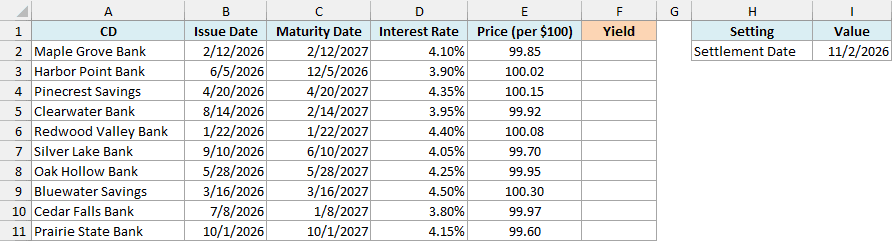
Below is a list of ten CDs offered on the secondary market, and I want the yield of each CD in column F, using the settlement date in I2.
Here is the formula:
=YIELDMAT(I2,+C2:C11,+B2:B11,+D2:D11,+E2:E11)
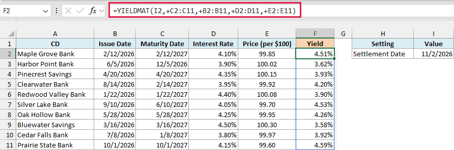
This one formula spills all ten yields into F2:F11. Each CD uses its own dates, interest rate, and price, while the settlement date in I2 applies to every CD.
The issue dates are in column B and the maturity dates in column C, because that’s the order they happen in. So the formula refers to C2:C11 before B2:B11, to match YIELDMAT’s argument order.
The plus sign (+) in front of each range is what makes the formula spill. YIELDMAT can’t take a range of cells directly, but the plus sign turns each range into a plain list of values, and YIELDMAT returns one result for each row.
It’s the same fix that works for other Excel functions that won’t spill, such as the EOMONTH and EDATE functions.
Important: Without the plus signs, YIELDMAT returns a single #VALUE! error instead of spilling. Put + in front of every range you pass to it, because leaving it off even one range breaks the results.
Look at the four CDs priced above 100: Harbor Point Bank, Pinecrest Savings, Redwood Valley Bank, and Bluewater Savings. Each one yields less than its interest rate, mainly because you lose the amount above 100 at maturity.
Harbor Point Bank shows how much the time left matters. At a price of 100 it would yield 3.84%, but at 100.02 it yields 3.62%.
That 0.02 loss is tiny, but it comes in about a month (the CD matures on December 5, 2026). Turned into an annual rate, it costs more than 0.2 percentage points.
If you are using Excel 2019 or earlier, enter the below formula in cell F2 and then copy it down the range:
=YIELDMAT($I$2,C2,B2,D2,E2)
Example 3: Rank CDs by Yield
Once you have the yields, the next question is usually which CD pays the most.
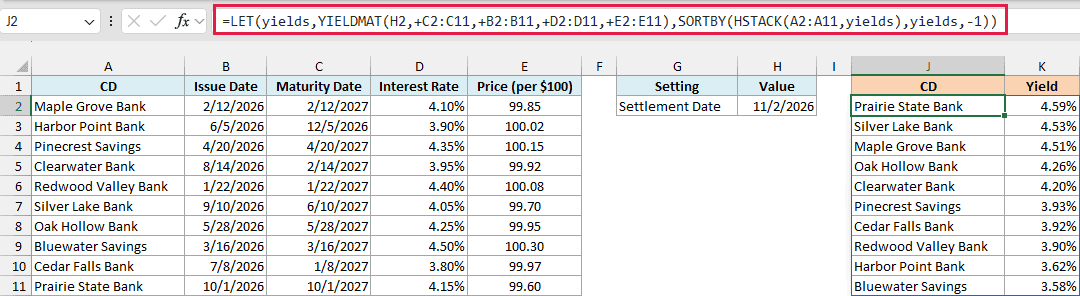
Below is the same list of ten CDs, and I want them sorted from the highest yield to the lowest in columns J and K.
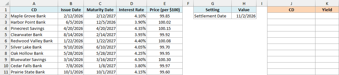
Here is the formula:
=LET(yields,YIELDMAT(H2,+C2:C11,+B2:B11,+D2:D11,+E2:E11),SORTBY(HSTACK(A2:A11,yields),yields,-1))
How this formula works:
- The LET function calculates the ten yields once, with the same YIELDMAT formula as Example 2 (the settlement date is in H2 this time), and stores them under the name
yields. That way, the rest of the formula can use them twice. HSTACK(A2:A11,yields)uses the HSTACK function to put the CD names next to their yields as a two-column list.SORTBY(...,yields,-1)uses the SORTBY function to sort that list by yield, from the highest to the lowest (the -1 means descending).
Prairie State Bank comes out on top at 4.59%. Bluewater Savings, which has the highest interest rate in the list (4.50%), comes last at 3.58%, because it costs 100.30.
So when you compare CDs, sort by yield rather than by the interest rate. And since the ranking is a formula, it updates on its own when you change a price.
Because the HSTACK function is only in Excel 365 and Excel 2024, this formula works only in those versions.
If you’re using an older version, go back to the list in Example 2, enter its Excel 2019 formula in F2, and copy it down.
Then select A1:F11 and sort it by the Yield column, largest to smallest, with the Sort option on the Data tab.
Example 4: Yield From a Trade Confirmation in Dollars
Sometimes all you have is the dollar amounts on your broker’s trade confirmation, not a price per $100.
Below is a confirmation for $25,000 of a CD, with the principal and the accrued interest (the interest built up since the issue date) shown separately, and I want the yield in cell B11.
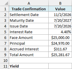
Here is the formula:
=YIELDMAT(B2,B3,B4,B5,B7/B6*100)
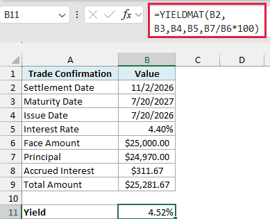
YIELDMAT needs the price per $100, so B7/B6*100 turns the principal into one. $24,970 for $25,000 of face value is a price of 99.88, and the formula returns 4.52%.
The principal is what you pay for the CD itself. The accrued interest ($311.67) goes to the seller for the interest the CD built up while they held it, and you get it back at maturity as part of the full interest payment.
If a confirmation doesn’t show the accrued interest, you can work it out with the ACCRINTM function. For this CD, it returns the same $311.67 from the issue date, the settlement date, the 4.40% rate, and the $25,000 face value.
Important: Use the principal, not the total amount, to work out the price. YIELDMAT already adds the accrued interest itself, so the $25,281.67 total counts it twice and returns 2.76% instead of 4.52%.
Example 5: Check the YIELDMAT Result by Hand
Here’s a quick way to see what YIELDMAT is measuring.
A CD that pays all its interest at maturity has only one payment left, so its yield is simply what you gain as a share of what you pay, turned into an annual rate.
Below is the CD from Example 1 with its YIELDMAT result in B8, and I want to work out the same yield by hand in cell B9.
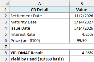
Here is the formula:
=LET(held,DAYS360(B4,B2),term,DAYS360(B4,B3),paid,B6+100*B5*held/360,received,100+100*B5*term/360,(received-paid)/paid*360/(term-held))
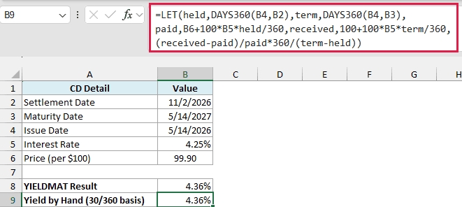
How this formula works:
heldandtermuse the DAYS360 function, which counts every month as 30 days (a 360-day year), the same as YIELDMAT’s default basis. That gives 168 days from the issue date to the settlement date, and 360 days from the issue date to maturity.paidis the price (99.90) plus the interest built up over those 168 days (1.98). That’s the 101.88 you actually hand over.receivedis the 100 you get back plus a full year of interest (4.25), so 104.25.(received-paid)/paidis your gain as a share of what you paid, which is about 2.32%.360/(term-held)turns that into an annual rate, based on the 192 days (in 30/360 terms) you hold the CD.
Both cells show 4.36%, so YIELDMAT is a simple annual return on what you pay. There’s no compounding, because there’s only one payment to wait for.
Because it uses the DAYS360 function, this check only matches YIELDMAT with the default basis of 0 (US 30/360). It’s a way to understand the result, and YIELDMAT is still the function to use.
The LET function used here works in Excel 365 and Excel 2021 or later.
Example 6: Highest Price to Pay for a Target Yield (PRICEMAT)
Let’s flip the question around: how much can you pay for a CD and still get the yield you want?
This CD was issued on June 10, 2026, matures a year later, and pays 4.00% at maturity, but I want a yield of 4.50%.
Below are the details of the CD with the target yield in B6, and I want the highest price I can pay in B8, and then a check of that price with YIELDMAT in B9.
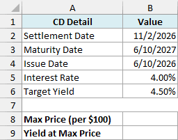
Here is the formula for the highest price:
=PRICEMAT(B2,B3,B4,B5,B6)
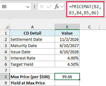
The PRICEMAT function is the reverse of YIELDMAT. It takes the same arguments, except that the yield goes where the price would be, and it returns the price per $100.
Here it returns 99.66. If you pay 99.66 or less for this CD, you get a yield of at least 4.50%.
And here is the YIELDMAT formula that checks it:
=YIELDMAT(B2,B3,B4,B5,B8)
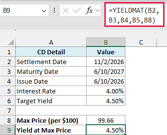
Putting that price back into YIELDMAT returns exactly 4.50%, which confirms the two functions agree.
The formula points at B8 rather than a typed 99.66. That’s because B8 holds the full unrounded price, and the rounded 99.66 would return 4.51%.
So these are six practical ways to use the YIELDMAT function in Excel. It gets you the real yield of a CD or note that pays its interest at maturity, and the PRICEMAT function gives you the price when you start from a target yield.
If a security pays its interest in regular coupons instead, use the YIELD function. If it pays no interest and sells at a discount, like a Treasury bill, the YIELDDISC function is the one you need.
I hope you found this Excel tutorial useful.
Other Excel Articles You May Also Like:
