AND Function in Excel (8 Examples)

If you want to check whether several conditions are all true at the same time, the AND function is what you’re looking for.

It returns TRUE only when every condition you give it is met, and FALSE as soon as even one of them fails.

One thing to know up front: AND always returns a single TRUE or FALSE. So it does not spill down a column the way many functions do in Excel 365.

In this article, I’ll walk you through the AND function with practical examples, from simple checks to using it inside IF, dynamic array formulas, and conditional formatting rules.

AND Function Syntax

Here is the syntax of the AND function:

=AND(logical1, [logical2], ...)

• logical1 – the first condition you want to test. This can be a comparison like B2>100, a cell that already holds TRUE or FALSE, or a range of logical values. Required.
• logical2, … – optional extra conditions to test. You can add up to 255 conditions in total.

The result is always a single value: TRUE if every condition is met, and FALSE if even one of them is not.

AND also treats numbers as logical values. Any number other than 0 counts as TRUE, and 0 counts as FALSE.

So =AND(5,1) returns TRUE, while =AND(5,0) returns FALSE because of that zero.

Pro Tip: If you hand AND a range that contains text or empty cells, those are ignored. But if the range has no logical values at all, AND returns a #VALUE! error.

When to Use the AND Function

Use the AND function when you need to:

• Check that several conditions are all true before you take an action
• Test whether a number falls between a lower and an upper limit
• Combine multiple tests inside an IF function to return your own custom results
• Build conditional formatting rules that only trigger when every condition is met

Let me show you a few practical examples of how this works.

Example 1: Check If Multiple Conditions Are All True

Let’s start with a simple example.

Below is an orders table with the order ID in column A, the order value in column B, whether the item is in stock in column C, and the shipping destination in column D.

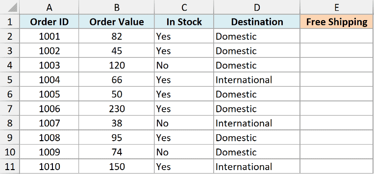
I want to flag which orders qualify for free shipping, which needs an order value of at least 50, the item in stock, and a domestic destination.

Here is the formula:

=AND(B2>=50, C2="Yes", D2="Domestic")

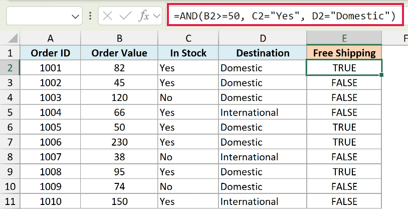
AND checks all three conditions for that row. The order value has to be 50 or more, the in-stock cell has to say Yes, and the destination has to be Domestic.

Only when all three are true does the formula return TRUE. If even one fails, you get FALSE. Copy it down the column to check every order.

Notice the text conditions “Yes” and “Domestic” are wrapped in double quotes, while the number comparison B2>=50 is not.

These text checks are not case-sensitive, so “yes”, “YES”, and “Yes” all pass the C2=”Yes” test.

Important: Wildcards don’t work in these comparisons. D2=”Dom*” looks for the literal text Dom*, so it won’t match “Domestic”.

If you need a partial match, you can use something like ISNUMBER(SEARCH("Dom",D2)) as the condition instead.

Here’s more on how wildcard characters work in Excel.

Example 2: Check If a Number Is Between Two Values

Here’s a really common use for AND: testing whether a value sits inside a range.

Below I have temperature readings from a cold-storage unit, with the reading time in column A and the temperature in Celsius in column B. The safe range for this unit is between 2 and 8 degrees.

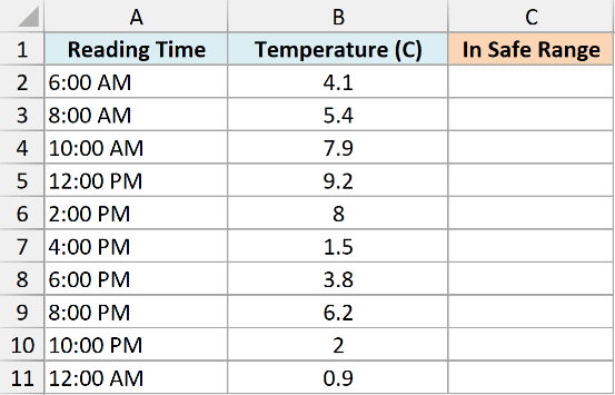
I want to check whether each reading is inside that safe band.

Here is the formula:

=AND(B2>=2, B2<=8)

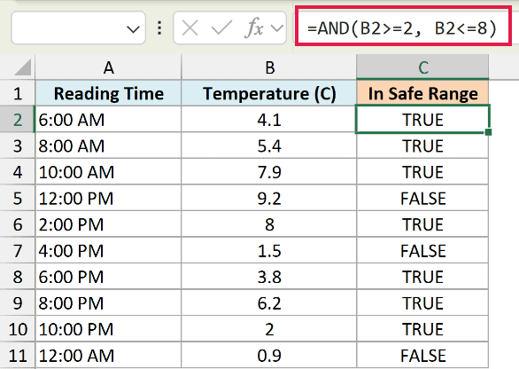
This is where AND really shines. A single cell can’t be greater than 2 and less than 8 in one comparison, so you need two separate tests joined together.

The first condition checks the reading is 2 or higher. The second checks it’s 8 or lower. A reading of 5.4 passes both and returns TRUE, while 9.2 fails the upper limit and returns FALSE.

The same two-test pattern works with dates too, which is handy when you need to check if a date is between two dates.

Example 3: Use AND Inside an IF Function

The AND function gets a lot more useful once you nest it inside IF. On its own AND only gives you TRUE or FALSE, but IF lets you return whatever text or number you want instead.

Below is a rental application table with the applicant in column A, their credit score in column B, annual income in column C, and whether they have a prior eviction in column D.

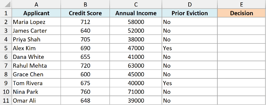
I want to mark an application as “Approve” only when the credit score is at least 650, income is at least 40000, and there is no prior eviction.

Here is the formula:

=IF(AND(B2>=650, C2>=40000, D2="No"), "Approve", "Manual Review")

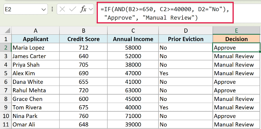
Here AND does the checking and IF does the labeling.

AND tests all three conditions and hands a single TRUE or FALSE back to IF. When it’s TRUE, IF returns “Approve”. When it’s FALSE, IF returns “Manual Review” instead of a bare FALSE.

An applicant with a 712 score, 58000 income, and no eviction passes all three tests, so this returns “Approve”.

Example 4: Combine AND with OR for Mixed Logic

Sometimes your rules aren’t all “must be true”. You need some conditions that are strict and one that can be satisfied a couple of different ways. That’s when you nest OR inside AND.

Below is a flight upgrade list with the passenger in column A, their loyalty tier in column B, seats available in column C, and their fare class in column D.

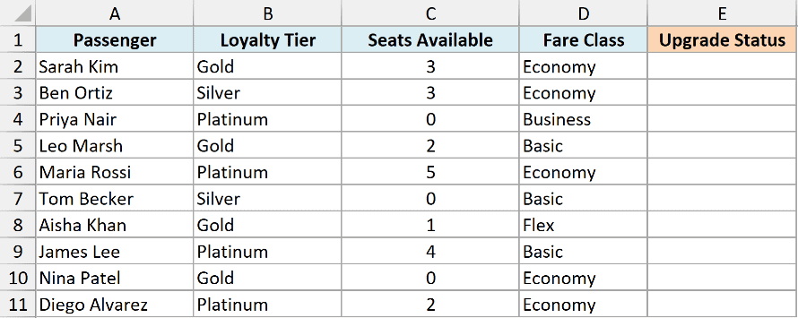
I want to mark a passenger “Eligible” when they are Gold or Platinum tier, there is at least one seat available, and their fare class is not Basic.

Here is the formula:

=IF(AND(OR(B2="Gold", B2="Platinum"), C2>0, D2<>"Basic"), "Eligible", "Not Eligible")

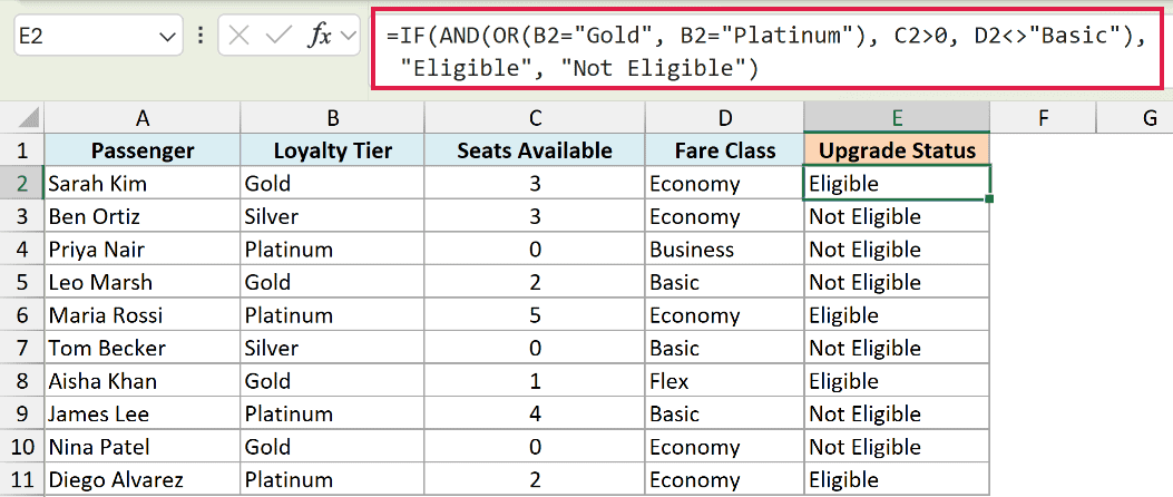
The OR part handles the tier. It returns TRUE if the passenger is Gold or Platinum, so either one counts.

That result then joins the other two AND conditions: a seat is free, and the fare class is anything other than Basic. All three parts of the AND have to be true for the passenger to come back “Eligible”.

A Gold passenger with 3 seats free on an Economy fare passes every check, so the formula returns “Eligible”.

Remember that AND needs all conditions met. If you only need one of several to pass, reach for the OR function instead.

And if you want to flip a result, wrap it in the NOT function.

Example 5: Apply AND Logic in a Dynamic Array Filter

Now let’s look at something modern. If you’re on Excel 365 or 2021, you’ll often want row-by-row AND logic across a whole range, usually to filter a list down to the rows that meet every condition.

There’s a catch here worth knowing. You can’t just drop the AND function inside FILTER. Writing AND(B2:B13>=20, ...) collapses the entire range into one TRUE or FALSE, so FILTER can’t tell the rows apart.

The fix is to multiply the conditions together with *. Multiplication works element by element, so it acts as an AND on each row without collapsing anything.

Below is a product list with the product name in column A, price in column B, and whether it’s in stock in column C.

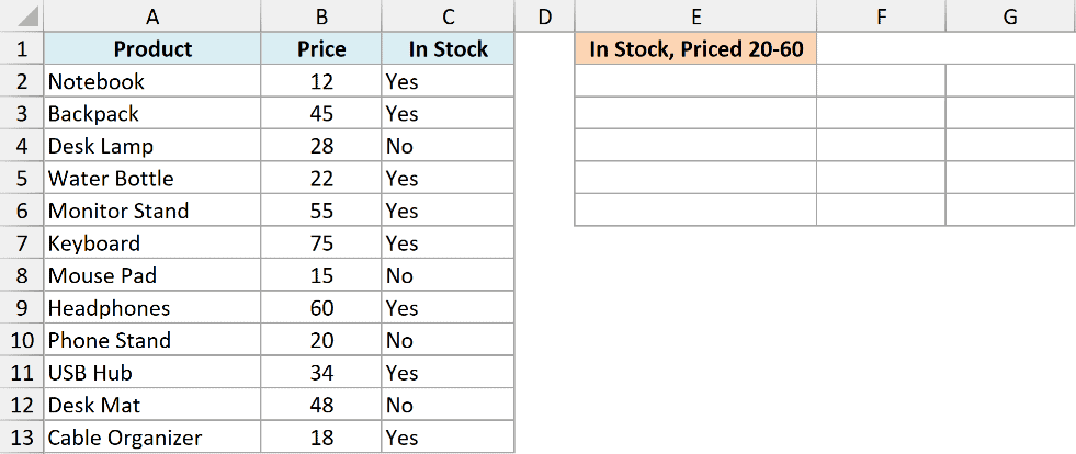
I want to pull out only the products priced between 20 and 60 that are also in stock.

Here is the formula:

=FILTER(A2:C13, (B2:B13>=20)*(B2:B13<=60)*(C2:C13="Yes"))

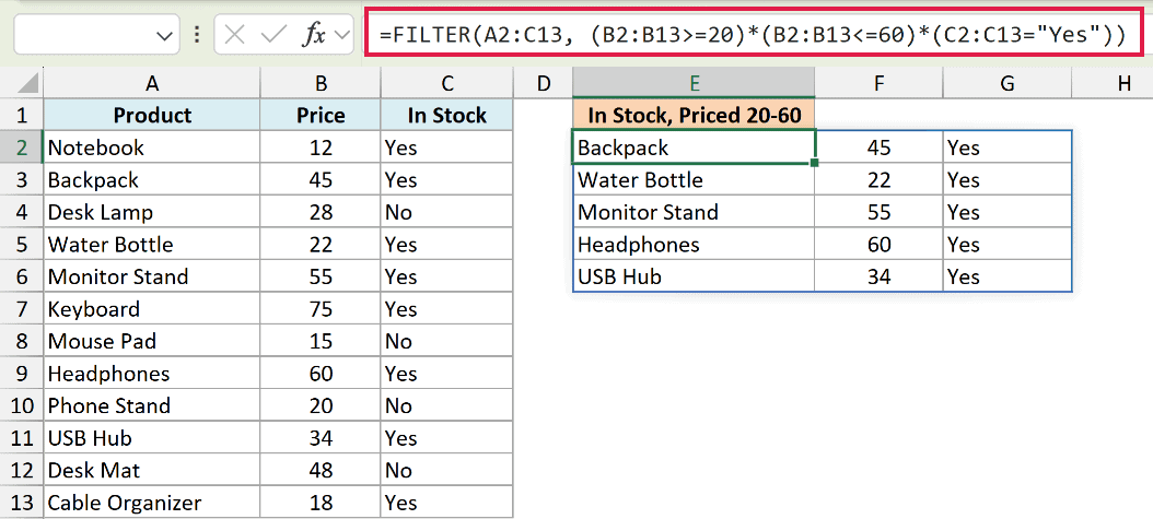
Each condition in parentheses produces a TRUE/FALSE array, one value per row.

Multiplying them turns TRUE into 1 and FALSE into 0, so a row only survives when all three come out as 1. FILTER keeps those rows and spills the matching products into the cells below.

Pro Tip: Use * between conditions for AND logic, and + for OR logic. The FILTER function and spill ranges need Microsoft 365 or Excel 2021, so this won’t work in Excel 2019 or earlier.

Example 6: Check If All Values in a Range Meet a Condition

So far, every formula has checked one row at a time. But sometimes you want a single yes or no answer for a whole list.

Below is a week of step counts from a fitness tracker, with the day in column A and the number of steps in column B.

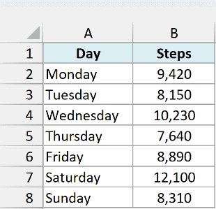
I want to check whether the 8,000-step goal was hit on every single day of the week.

Here is the formula:

=AND(B2:B8>=8000)

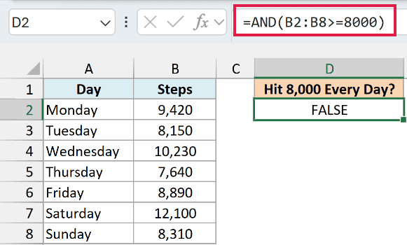
The B2:B8>=8000 part compares every cell in the range with 8,000, which gives AND seven TRUE or FALSE values. AND then boils them all down to one answer for the whole range, not one per row.

Thursday only has 7,640 steps, so the formula returns FALSE. If every day had 8,000 steps or more, you’d get TRUE.

Important: In Excel 365 and 2021, just press Enter. In Excel 2019 or older, confirm this formula with Control + Shift + Enter, or it won’t check the whole range.

If your column already holds TRUE or FALSE values (like a task checklist), you can skip the comparison and use =AND(B2:B8) directly.

Example 7: Use AND with Dates

AND works with dates too, since Excel stores every date as a number in the back end.

Below is a list of library books, with the book name in column A, the due date in column B, and the date it was returned in column C.

A blank in column C means the book hasn’t come back yet.

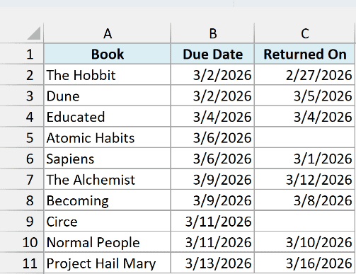
I want to check which books were returned on or before their due date.

Here is the formula:

=AND(C2<>"",C2<=B2)

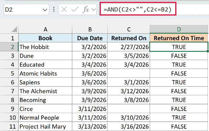
The second condition does the real check. The return date in column C has to be on or before the due date in column B.

The first condition is there for books that haven’t come back. Excel treats a blank cell as 0, and 0 is smaller than any date.

So without C2<>””, a book like Atomic Habits (no return date) would wrongly show up as returned on time. With it, those rows return FALSE.

Example 8: Use AND in Conditional Formatting

AND is also really handy inside conditional formatting, when you want to highlight rows that meet several conditions at once.

Below is a list of apartment listings, with the apartment in column A, the city in column B, the monthly rent in column C, and the number of bedrooms in column D.

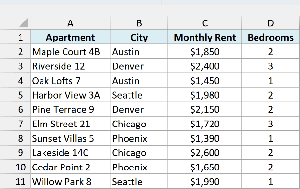
I want to highlight every apartment that rents for $2,000 or less and has at least 2 bedrooms.

Here are the steps to do this:

1. Select the data without the headers (A2:D11 here)

2. Click the Home tab

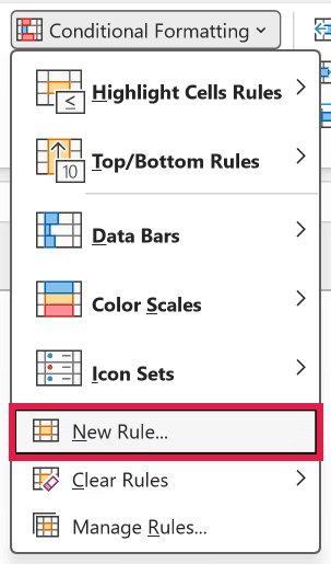
3. In the Styles group, click on Conditional Formatting

4. Click on New Rule

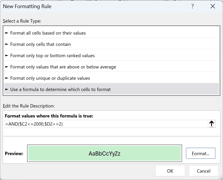
5. In the New Formatting Rule dialog box, click on ‘Use a formula to determine which cells to format’

6. In the formula field, enter =AND($C2<=2000,$D2>=2)

7. Click the Format button

8. In the Fill tab, pick a light green color and click OK

9. Click OK

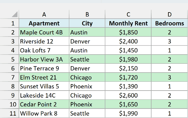
Every row where the rent is $2,000 or less and there are 2 or more bedrooms is now highlighted.

The $ sign before C and D locks the columns, while the row number stays relative. So each row checks its own rent and bedrooms, and the whole row gets the color.

If you want to go further with this, here’s my guide on how to highlight an entire row based on a cell value.

AND Function vs & (Ampersand) in Excel

Since & is often read as “and”, it’s easy to assume it works like the AND function. But in Excel, the & symbol joins text together.

For example, =A2&" "&B2 combines a first name in A2 and a last name in B2 with a space in between.

It works just like the CONCATENATE function and doesn’t test any conditions.

For AND logic, use the AND function, or multiply conditions with * inside array formulas like FILTER (as shown in Example 5).

Wrapping Up

The AND function is a small but handy tool once it clicks. We covered checking several conditions at once, testing whether a number sits between two values, and using AND inside IF, OR, and dynamic array formulas.

We also checked a whole range at once, worked with dates, and highlighted rows with conditional formatting.

I hope you found this tutorial helpful.

List of All Excel Functions

Other Excel Articles You May Also Like:

• IFS Function in Excel
• Excel NOT Function