

You used COUNT and COUNTA on the same range, but they returned two different numbers.
The difference between COUNT and COUNTA is that COUNT counts cells with numbers, while COUNTA counts every cell that isn’t empty.
That sounds simple, but cells that only look empty and numbers stored as text can give you a count you didn’t expect.
In this article, I’ll show you which function to use, the traps to watch for, and how to use both together.
Both return a single number, but they also work inside dynamic array formulas, such as =COUNTA(UNIQUE(...)).
Follow along with the example file
COUNT vs COUNTA Examples.xlsx
COUNT vs COUNTA: The Quick Answer
COUNT answers “How many numbers are in here?”
COUNTA answers “How many cells have anything in them?“
Here is what each function counts when you give it a range of cells:
| Cell contains | COUNT | COUNTA |
|---|---|---|
| Number (450) | ✅ | ✅ |
| Date (3/5/2026) | ✅ | ✅ |
| Time (9:30 AM) | ✅ | ✅ |
| Number stored as text ("450") | ❌ | ✅ |
| Text ("Pending") | ❌ | ✅ |
| TRUE / FALSE | ❌ | ✅ |
| Error value (#N/A) | ❌ | ✅ |
| Formula that returns "" | ❌ | ✅ |
| A single space | ❌ | ✅ |
| Truly empty cell | ❌ | ❌ |
Dates and times count as numbers because Excel stores them as numbers. The only thing COUNTA skips is a truly empty cell.
Below is the Data Types sheet, with the cell descriptions in column A, example values in B, and COUNT and COUNTA results in C and D.
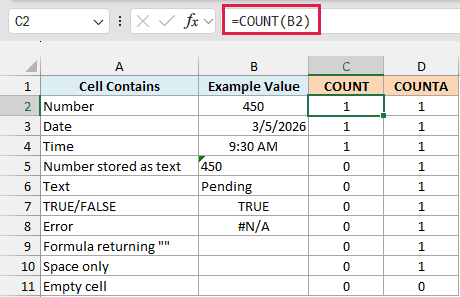
Each row checks a single cell. A result of 1 means the cell was counted, and 0 means it was skipped.
For example, C2 uses =COUNT(B2) and D2 uses =COUNTA(B2). The same check runs down to row 11, so you can see each difference separately.
COUNT and COUNTA Syntax
Both functions have the same argument structure. Here is the COUNT syntax:
=COUNT(value1, [value2], ...)
And here is the COUNTA syntax:
=COUNTA(value1, [value2], ...)
- value1 is required. It can be a cell, a range, or a value you type into the formula.
- value2 and any further arguments are optional. Add them when you want to include more cells, ranges, or values.
- Both functions accept up to 255 arguments. A range counts as one argument, regardless of how many cells it contains.
You can give either function one range, several ranges, or typed values. Most of the time, you’ll point it at a range.
Values typed directly into COUNT are treated differently from values inside cells.
For example, =COUNT(1,"5",TRUE,"x") returns 3. It counts 1, the number written as text, and TRUE when they’re typed directly into the formula.
Inside cells, COUNT skips that text number and TRUE. Meanwhile, =COUNTA(1,"5",TRUE,"x","") returns 5, including the empty text at the end.
When to Use COUNT and When to Use COUNTA
Pick the function based on what you need the count to tell you:
- Use COUNT to check how many sales amounts or scores were entered, how many tasks have a completion date, or how many numeric prices a lookup found.
- Use COUNTA to count names or entries in a list, responses regardless of what was typed, or items returned by a dynamic array formula.
If a column should contain only numbers, compare COUNT with COUNTA to check for bad entries. Examples 2 and 6 show how that comparison works.
Let me show you how these differences play out with a few practical examples.
Example 1: COUNT vs COUNTA, Same Column
Let’s start with a column that contains both amounts and text.
The Same Column sheet has fun-run runners in A2:A11 and sponsorship pledges in B2:B11.
Seven runners have dollar amounts, Aisha and Mateo show “Pending”, and Oliver’s pledge is blank. The result cells B13 and B14 start empty below the list.
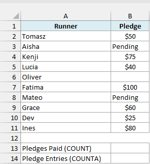
I want to count how many runners have paid, then compare that with how many have anything recorded in the Pledge column.
Enter this COUNT formula in B13, beside “Pledges Paid (COUNT)”:
=COUNT(B2:B11)
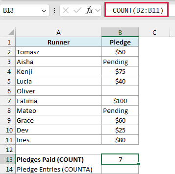
This returns 7. COUNT includes the seven dollar amounts and skips both “Pending” entries and Oliver’s blank cell.
Now enter this COUNTA formula in B14, beside “Pledge Entries (COUNTA)”:
=COUNTA(B2:B11)
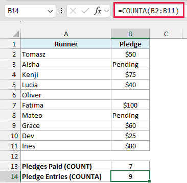
This returns 9, because COUNTA includes the two “Pending” entries too. It skips only Oliver’s blank pledge.
Both answers are correct. Seven people have paid, while nine runners have something recorded. The difference of 2 is the two pending pledges.
Example 2: Find Numbers Stored as Text
Now let’s look at a column where everything looks like a number, but COUNT still skips some entries.
The Numbers as Text sheet contains a step-tracker export in A1:B11, covering March 2 to March 11, 2026.
Dates are in column A and steps in B. The summary labels are in A13:A15, with empty result cells in B13:B15.
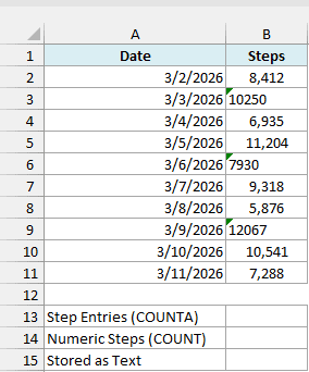
I want to compare the number of filled step entries with the number Excel recognizes as numeric.
First, enter this formula in B13 to count the entries:
=COUNTA(B2:B11)
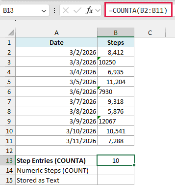
COUNTA returns 10, since all 10 cells contain something.
Next, enter this formula in B14 to count the numeric entries:
=COUNT(B2:B11)
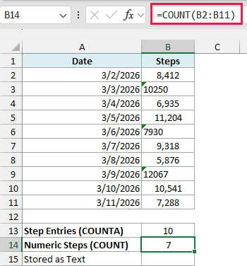
COUNT returns 7. The values 10250, 7930, and 12067 are stored as text, so it quietly skips them.
Notice that those three entries sit on the left and have no thousands separator. The real numbers use the 8,412 format.
A SUM or AVERAGE on this range would also leave those three text entries out.
To find the number of non-numeric entries, enter this formula in B15:
=COUNTA(B2:B11)-COUNT(B2:B11)
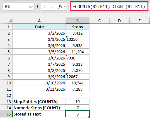
This returns 3. In a column that should contain only numbers, any result other than 0 tells you something needs fixing.
COUNTA minus COUNT includes every filled cell that isn’t a number, including text, TRUE/FALSE, and errors. It doesn’t specifically identify numbers stored as text.
In this export, all three non-numeric entries are text numbers. If other types of junk are possible, =SUMPRODUCT(--ISTEXT(B2:B11)) counts only text, also 3 here.
Data imported from another system often arrives as text. Convert those entries to numbers so COUNT, SUM, and AVERAGE can use them.
The same applies to dates. COUNT includes real Excel dates, but skips a date imported as text.
Example 3: Count Cells That Look Blank
A cell can look empty and still be counted by COUNTA, as this rental example shows.
The Looks Blank sheet has cars in A2:A11, Days Rented in B, Daily Rate in C, and Rental Total in D.
Days Rented is blank for cars still out. In D2, =IF(B2:B11="","",B2:B11*C2:C11) spills the totals down to D11.
Six cells show amounts: $135, $445, $120, $665, $200, and $46. The other four look empty because the formula returns "", an empty string.
The summary labels are in A13:A15, and I’ll enter the counting formulas in the empty cells B13:B15.
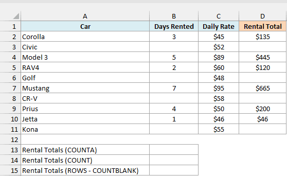
I want to count how many rentals have an actual total, leaving out the four cells that only look blank.
Start with COUNTA in B13:
=COUNTA(D2:D11)
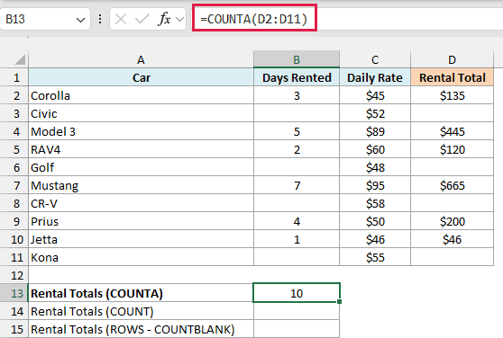
This returns 10, which is the wrong count for our goal. COUNTA counts the four empty strings along with the six amounts.
Those cells aren’t truly empty. They contain text returned by a formula, even though that text has no visible characters.
Since our totals are numbers, enter COUNT in B14:
=COUNT(D2:D11)
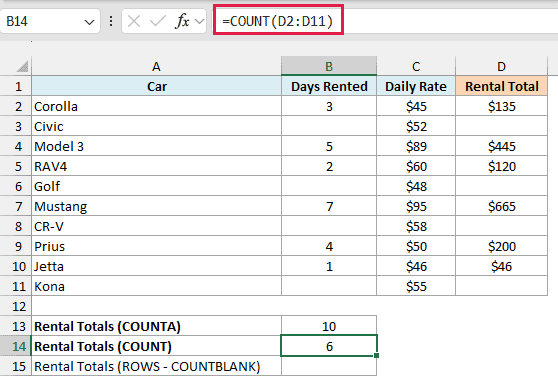
This gives the correct result, 6. COUNT includes the numeric totals and ignores the empty strings because they’re text.
But COUNT wouldn’t help if the formula returned “Returned” instead of an amount. To count either text or numbers while excluding "", enter this in B15:
=ROWS(D2:D11)-COUNTBLANK(D2:D11)
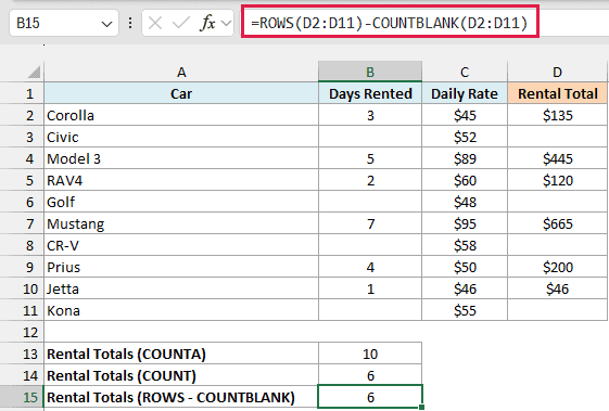
This also returns 6. ROWS gives us the 10 cells in this single-column range, and COUNTBLANK counts the four empty strings. Subtracting gives 6.
Important: The common non-blank formula =COUNTIF(D2:D11,"<>") has the same problem as COUNTA here. It also returns 10.
COUNTA and COUNTBLANK both count the "" cells. So COUNTA (10) plus COUNTBLANK (4) gives 14, even though the range has only 10 cells.
A cell containing a single space also looks empty, and COUNTA counts it. COUNTBLANK doesn’t treat a space as blank, so ROWS minus COUNTBLANK won’t help there.
The spilling IF formula needs Excel 365 or Excel 2021 or later. In older versions, enter =IF(B2="","",B2*C2) in D2 and copy it down.
Example 4: Count TRUE/FALSE Values
Let’s try an attendance list, where the entries are TRUE and FALSE instead of numbers or text.
The TRUE FALSE sheet has 10 volunteers in A2:A11 and their attendance in B2:B11.
Seven volunteers have TRUE and three have FALSE. The summary labels are in A13:A15, and the result cells B13:B15 start empty.
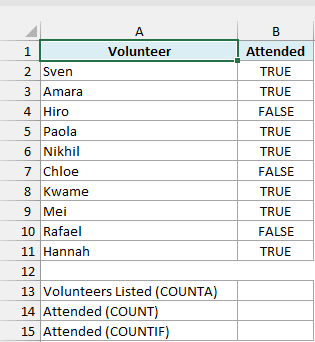
I want to count only the volunteers who attended, which means counting the TRUE values.
First, enter COUNTA in B13:
=COUNTA(B2:B11)
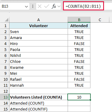
This returns 10. COUNTA counts both TRUE and FALSE, so it tells us how many volunteers have an attendance status.
Now enter COUNT in B14:
=COUNT(B2:B11)
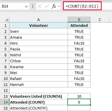
This returns 0. COUNT ignores TRUE/FALSE values inside cells, even though Excel can treat TRUE as 1 and FALSE as 0 in calculations.
To count only those who attended, enter COUNTIF in B15:
=COUNTIF(B2:B11,TRUE)
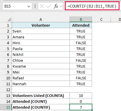
This returns 7, the correct attendance count. COUNTIF checks the condition and counts only the cells containing TRUE.
In Microsoft 365, you can add in-cell checkboxes using Insert > Checkbox. A checked box stores TRUE, and an unchecked box stores FALSE.
Pro Tip: Use =COUNTIF(range,TRUE) to count checked in-cell checkboxes. COUNT returns 0 for a column of these checkboxes.
Example 5: Count Cells With Errors
Errors are another kind of entry COUNTA includes, which matters when you’re checking lookup results.
The Errors sheet has a plant order in A1:B11 and a price list in D1:E8. The result cells B13:B14 are below the order.
Column A lists the ordered plants. In B2, =XLOOKUP(A2:A11,D2:D8,E2:E8) looks up their prices and spills the results down to B11.
Orchid, Bonsai, and Rosemary aren’t in the price list, so B4, B7, and B11 show #N/A. The summary result cells B13:B14 start empty.
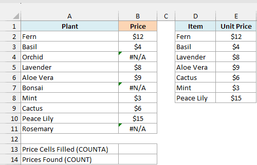
I want to count how many plants actually got a price, excluding the three lookup errors.
Enter COUNTA in B13, beside “Price Cells Filled (COUNTA)”:
=COUNTA(B2:B11)
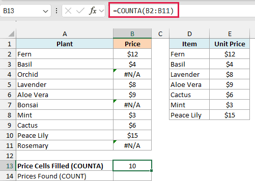
This gives 10. An error is still something in a cell, so COUNTA counts the three #N/A results along with the seven prices.
For the number of prices found, enter COUNT in B14:
=COUNT(B2:B11)
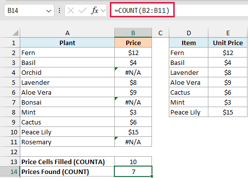
COUNT returns 7. It includes the numeric prices and ignores the errors, giving us the count we wanted.
Here, COUNTA minus COUNT gives 3, the number of plants missing from the price list.
You can give XLOOKUP a fourth argument such as “Not found” to display text instead of #N/A. Here I’ve left it out so you can see how each function treats errors.
XLOOKUP needs Excel 365 or Excel 2021 or later. In older versions, VLOOKUP also returns #N/A when it can’t find an item using an exact match.
Example 6: Use COUNT and COUNTA Together
You can also use the two functions on different columns to track how much work is left.
The Use Together sheet has 12 swimmers in A2:A13 and trial times in B2:B13.
Eight swimmers have a time recorded. Zara, Brooke, Arjun, and Noor have blank time cells because they haven’t swum yet.
The labels “Still to Swim (COUNTA – COUNT)” and “Percent Done (COUNT / COUNTA)” are in A15:A16, with empty result cells in B15:B16.
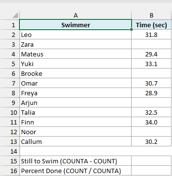
I want to count the swimmers still waiting, then calculate how far through the trials we are.
Enter this formula in B15:
=COUNTA(A2:A13)-COUNT(B2:B13)
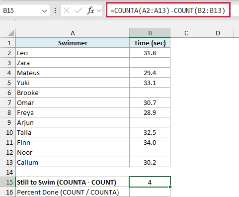
This returns 4. COUNTA counts the 12 names, and COUNT counts the 8 numeric times. Subtracting gives the swimmers still waiting.
For the completion percentage, enter this formula in B16 and format the cell as a percentage with no decimal places:
=COUNT(B2:B13)/COUNTA(A2:A13)
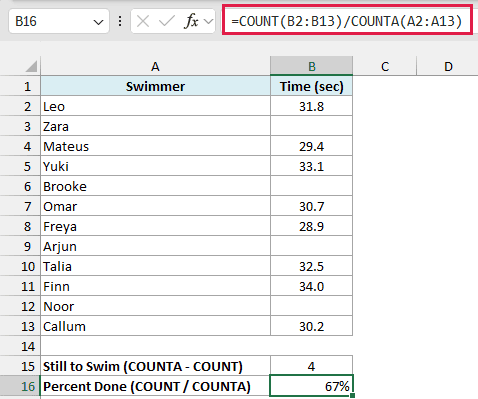
This shows 67%, which is 8 out of 12 rounded to a whole percentage.
COUNTA on the name column gives the size of the list. COUNT on the time column gives how many swimmers are done.
The results update as you enter times within these ranges. If you add swimmers beyond row 13, expand both ranges to include their names and times.
=COUNTBLANK(B2:B13) also returns 4 here. But a larger range would include empty rows below the last swimmer, while COUNTA minus COUNT stays tied to the names.
Keep the recorded times numeric. A time entered as text would be skipped by COUNT, so that swimmer would still appear to be waiting.
Example 7: COUNTA With Dynamic Array Formulas
Finally, let’s count items returned by another formula, where a no-match result needs a little care.
The Dynamic Arrays sheet has 12 hostel guests in A2:A13, their countries in B, and nights stayed in C.
The summary labels are in A15:A17, with empty result cells in B15:B17. The longest stay in the guest list is 6 nights.
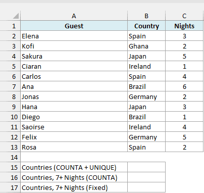
First, I want to count how many different countries the guests came from.
Enter this formula in B15:
=COUNTA(UNIQUE(B2:B13))
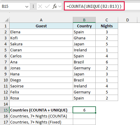
This returns 6. UNIQUE returns Spain, Ghana, Japan, Ireland, Brazil, and Germany, and COUNTA counts those six items.
COUNT wouldn’t work here because the country names are text.
Now I want the number of countries with a guest staying 7 or more nights. Nobody stayed that long, so the answer should be 0.
Enter this formula in B16 to see the problem:
=COUNTA(UNIQUE(FILTER(B2:B13,C2:C13>=7)))
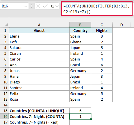
The result is 1, which is wrong. FILTER finds no matches and returns a #CALC! error. COUNTA then counts that error as one item.
To get the correct count, enter this formula in B17:
=IFERROR(ROWS(UNIQUE(FILTER(B2:B13,C2:C13>=7))),0)
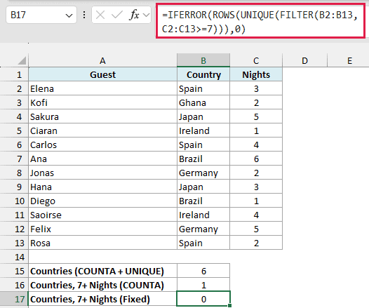
This returns 0. FILTER selects the matching countries, UNIQUE removes duplicates, and ROWS counts the rows in that list.
When there are no matches, the inner formula returns an error. IFERROR handles that no-match error and returns 0.
If you change the threshold to one with matches, such as 4 nights, the same approach counts the countries in the returned list.
Important: Giving FILTER an empty result of “” doesn’t fix COUNTA. =COUNTA(FILTER(...,"")) still returns 1 because it counts the empty string.
COUNT doesn’t have this issue with numbers. For example, =COUNT(FILTER(C2:C13,C2:C13>=7)) returns 0 because COUNT ignores the no-match error.
IFERROR would also hide other errors, such as a typo in the ranges. Check the formula when it shows 0, rather than assuming there are no matches.
UNIQUE and FILTER need Excel 365 or Excel 2021 or later. In older versions, =SUMPRODUCT(1/COUNTIF(B2:B13,B2:B13)) counts the distinct countries, also 6 here.
COUNT vs COUNTA in the Status Bar, Pivot Tables, and SUBTOTAL
You can see the same difference without typing COUNT or COUNTA into a cell.
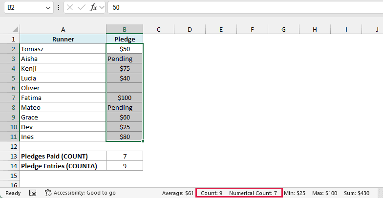
When you select cells, Excel’s status bar can show Count and Numerical Count. Count works like COUNTA, while Numerical Count works like COUNT.
If you don’t see Numerical Count, right-click the status bar and tick it.
Below is the Pledge range B2:B11 from Example 1 selected. The status bar shows Count 9 and Numerical Count 7.
In a pivot table’s Value Field Settings, Count works like COUNTA and Count Numbers works like COUNT.
A pivot table uses Count by default when the field contains text or blanks. Choose Count Numbers when you want only numeric entries included.
For filtered lists, SUBTOTAL(2,range) is the COUNT version and SUBTOTAL(3,range) is the COUNTA version. Both skip rows hidden by a filter.
I’ve shown you how COUNT and COUNTA differ, which cases can trip them up, and how to use them together.
I hope you found this article helpful.
Other Excel Articles You May Also Like:
- Count Cells That Are Not Blank in Excel
- COUNTIF Function in Excel (8 Examples)
- FILTER Function in Excel (10 Examples)
- SUBTOTAL Function in Excel
- COUNTIFS Function in Excel (9 Examples)
- ROWS Function in Excel (6 Examples)
- IS Functions in Excel (8 Examples)
- How to Count Cells that Contain Text Strings
