

The GESTEP function checks whether a number is greater than or equal to a threshold. It returns 1 when it is and 0 when it isn’t, so every value gets a flag that you can count or add up.
You can get the same yes-or-no answer with a >= comparison or an IF formula, so GESTEP is not the only way to do this.
GESTEP also checks one number at a time, so it returns an error when you give it a whole range. Example 2 shows a one-character fix for that.
In this article, I’ll show you where GESTEP fits, with five examples and a comparison with IF and the >= operator at the end.
Follow along with the example file
GESTEP Function Examples.xlsx
GESTEP Function Syntax
Here is the syntax of the GESTEP function:
=GESTEP(number, [step])
- number – The value you want to test. This one is required.
- step – The threshold you want to compare it with. This one is optional, and if you leave it out, Excel uses 0.
If the number is exactly equal to the step, GESTEP still returns 1. So =GESTEP(40,40) returns 1, because reaching the threshold counts.
Because step defaults to 0, a formula like =GESTEP(A2) checks whether A2 is zero or higher. It returns 1 for 0 and for any positive number, and 0 for a negative one.
Both arguments need to be numbers, although text that looks like a number (such as “5”) is fine. Other text, like “abc”, or a TRUE/FALSE value returns the #VALUE! error.
The GESTEP function works in Excel for Microsoft 365, Excel 2024, 2021, 2019, 2016, and Excel for Mac.
When to Use the GESTEP Function
Use this function when you need to:
- Flag every value that reaches a target or a pass mark with a 1 or a 0
- Count how many values hit a goal by adding up the 1s
- Work out what share of days or items met a target
- Add a charge or a bonus each time a value reaches another threshold
Let me show you a few practical examples of how to use the GESTEP function.
Example 1: Check If Each Value Reaches a Target
Let’s start with a simple example.
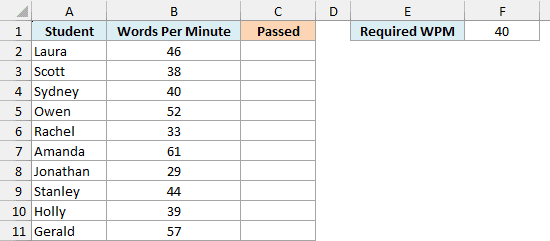
Below is the result of a typing test for a class, and I want to check in column C whether each student reached the required speed in cell F1.
Here is the formula to enter in cell C2 and copy down:
=GESTEP(B2,$F$1)
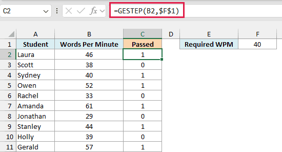
GESTEP compares the typing speed in B2 with the required speed in F1. If the student typed 40 words per minute or more, it returns 1, and otherwise it returns 0.
Sydney typed exactly 40 and still gets a 1, because a number that equals the step counts as reaching it. The dollar signs lock the reference to F1, so it doesn’t move as you copy the formula down.
I’ve used a per-row formula here because GESTEP doesn’t accept a whole range directly. The next example shows how to get around that with a single formula.
Example 2: Flag a Whole Column with One GESTEP Formula
Copying a formula down works fine, but in Excel 365 you’d usually want one formula that handles the whole column.
Below is a workout log with the minutes exercised each day, and I want to check in column C whether each day reached the daily target in cell F1.
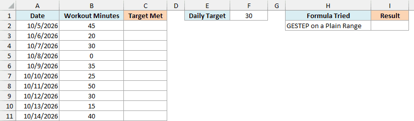
The natural first try is to give GESTEP the whole range of minutes. I’ve put that attempt in cell I2, and it returns a #VALUE! error:
=GESTEP(B2:B11,$F$1)
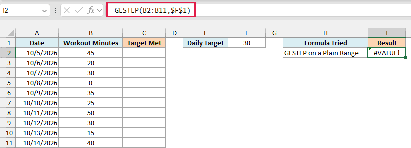
This happens because GESTEP can’t take a range reference like B2:B11 directly. It works only with numbers, or with a list of numbers held in memory (called an array).
Putting a plus sign (+) in front of the range fixes this, because Excel then turns the range into an array of values that GESTEP can work with. Here is the formula that works:
=GESTEP(+B2:B11,$F$1)
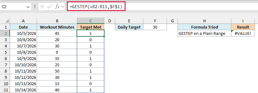
Enter this in cell C2, and the results fill down to C11 on their own, a 1 or a 0 for each day. Excel calls this spilling.
The two days with exactly 30 minutes get a 1, since reaching the target counts.
The same plus sign trick works for the DELTA function, which checks whether two numbers are equal and also refuses a plain range.
If you are using Excel 2019 or earlier, enter the below formula in cell C2 and then copy it down the range:
=GESTEP(B2,$F$1)
Important: A plain range like B2:B11 gives #VALUE! in every GESTEP formula, not just this one. Always put the plus sign in front of a range you pass as the number or the step.
Example 3: Leave Out the Step to Compare with Zero
Here’s another practical scenario.
Below is a small shop’s daily profit or loss, and I want to flag in column C the days that were not a loss.
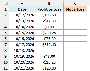
Here is the formula:
=GESTEP(+B2:B11)
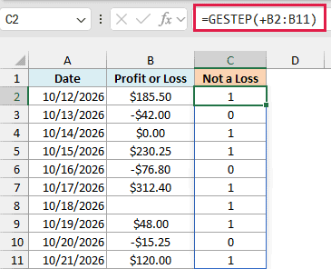
Since I’ve left out the step, GESTEP compares each value with 0. A profit returns 1, a loss returns 0, and the day that broke even at exactly $0.00 returns 1 as well.
The shop was closed on 10/18, so that cell is empty, and it also returns 1. GESTEP treats an empty cell as 0, which means a missing value looks the same as a break-even day.
If you are using Excel 2019 or earlier, enter the below formula in cell C2 and then copy it down the range:
=GESTEP(B2)
Important: If an empty cell means the value is missing, not zero, GESTEP still returns 1 for it. Check the blanks before you trust the result.
Example 4: Count Days That Hit a Goal with GESTEP and SUM
Since every day that hits the goal gets a 1, you can add up the results to count them.
Below is a 12-day log of the glasses of water someone drank, with the daily goal in cell E1, and I want to count the days that reached the goal in cell B15.
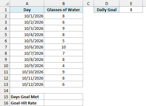
Here is the formula:
=SUM(GESTEP(+B2:B13,$E$1))
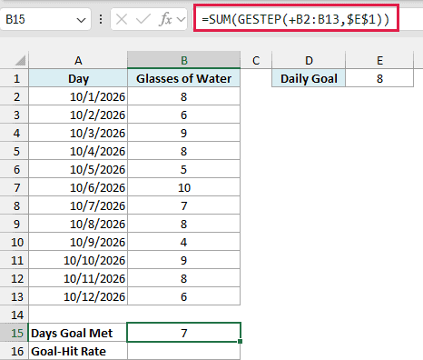
This returns 7, as seven of the twelve days reached the goal of 8 glasses.
GESTEP returns an array of twelve 1s and 0s, one for each day, and the SUM function adds that array up. The plus sign is there for the same reason as in Example 2.
Because the results are 1s and 0s, their average is the share of days that hit the goal. Here is the formula to enter in cell B16:
=AVERAGE(GESTEP(+B2:B13,$E$1))
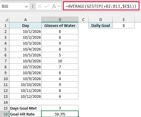
This returns 58.3%, which is 7 days out of 12. The cell is formatted as a percentage, so you see 58.3% instead of 0.583.
If you are using Excel 2019 or earlier, enter the below formula in cell B15 to count the days:
=COUNTIF(B2:B13,">="&$E$1)
And enter the below formula in cell B16 to get the share of days:
=COUNTIF(B2:B13,">="&$E$1)/COUNT(B2:B13)
The COUNTIF function is the shorter choice when a count is all you need, even in Excel 365. GESTEP earns its place when you want the 1s and 0s themselves, or an average of them.
Example 5: Add Step-Up Charges with GESTEP and SUMPRODUCT
Now let’s look at something more interesting.
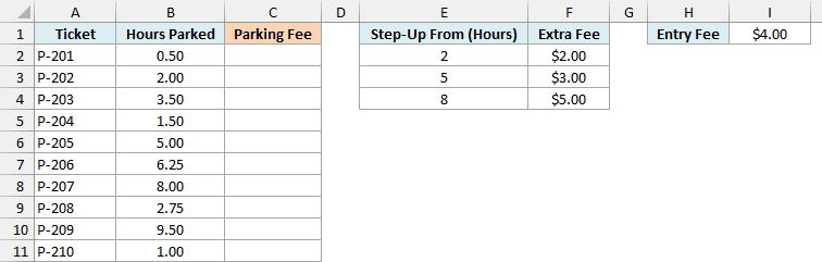
Below is a list of parking tickets with the hours parked, and I want to calculate the fee in column C.
The entry fee is in cell I1, and each extra fee in F2:F4 is added once the car has been parked for at least the step-up hours beside it in E2:E4.
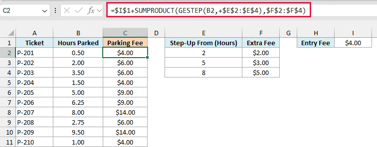
Here is the formula to enter in cell C2 and copy down:
=$I$1+SUMPRODUCT(GESTEP(B2,+$E$2:$E$4),$F$2:$F$4)
Here is how this formula works:
- GESTEP(B2,+$E$2:$E$4) compares the hours in B2 with each step-up hour (2, 5, and 8) and returns three flags. A car parked for 3.5 hours gets 1, 0, 0.
- SUMPRODUCT(…,$F$2:$F$4) multiplies each flag by its extra fee and adds them up. Only the step-up hours the car has reached add a charge.
- $I$1+ adds the $4.00 entry fee in front.
The plus sign in front of $E$2:$E$4 is there for the same reason as in Example 2. This time the step is the range, and the number is a single cell.
So P-203, parked for 3.5 hours, pays $4.00 + $2.00 = $6.00. P-207 was parked for exactly 8 hours, so it has reached all three step-up hours and pays $4.00 + $2.00 + $3.00 + $5.00 = $14.00.
If you change a step-up hour or a fee in E2:F4, every ticket updates on its own.
If you are using Excel 2019 or earlier, enter the below formula in cell C2 and then copy it down the range:
=$I$1+SUMIF($E$2:$E$4,"<="&B2,$F$2:$F$4)
This SUMIF formula gives the same fees. It adds the extra fee for every step-up hour that is less than or equal to the hours parked.
GESTEP vs IF vs the >= Operator
GESTEP is one of several ways to run the same test. Below, a typing speed of 40 words per minute in cell F1 is checked against a required 40 in cell F2, written five different ways (it’s the last sheet in the example file).
| Method | Formula | Returns |
|---|---|---|
| GESTEP | =GESTEP($F$1,$F$2) | 1 |
| IF returning 1 or 0 | =IF($F$1>=$F$2,1,0) | 1 |
| IF returning words | =IF($F$1>=$F$2,"Pass","Fail") | Pass |
| Comparison operator | =$F$1>=$F$2 | TRUE |
| Double negative | =--($F$1>=$F$2) | 1 |
The double negative (–) turns TRUE and FALSE into 1 and 0, so it gives the same result as GESTEP. It is shorter, and it works on a whole range without a plus sign.
Use IF when you want words like Pass or Fail, and the >= operator when TRUE or FALSE is enough.
There is one more difference with decimals. Excel stores numbers like 0.1 and 0.2 in binary, so adding them can leave a tiny leftover.
GESTEP reacts to that leftover and the >= operator doesn’t. For example, =GESTEP(0.3,0.1+0.2) returns 0, while =0.3>=0.1+0.2 returns TRUE.
If a value comes from decimal math, wrap it in the ROUND function. =GESTEP(0.3,ROUND(0.1+0.2,2)) returns 1.
Wrapping Up
The GESTEP function turns a threshold check into a 1 or a 0, which you can copy down, count with SUM, or average.
Remember that a value equal to the step counts, that an empty cell counts as 0, and that a range needs a plus sign in front of it.
I hope you found this tutorial useful.
Other Excel Articles You May Also Like:
