CHOOSE Function in Excel

The CHOOSE function in Excel returns an item from a list based on its position number. So if you give it 2, it returns the second item from your list of choices.

It’s handy for turning number codes like 1, 2, and 3 into labels without building a lookup table.

In this article, I’ll show you how to use the CHOOSE function in Excel with six practical examples.

Excel CHOOSE Function Syntax

Here is the syntax of the CHOOSE function:

=CHOOSE(index_num, value1, [value2], ...)

• index_num – Required. The position you want to return. It can be a number, a cell reference, a formula, or an array of numbers.
• value1 – Required. The first choice. Choices can be numbers, text, cell references, ranges, defined names, or formulas.
• [value2], … – Optional additional choices. You can supply up to 254 values in total, including value1.

CHOOSE counts from 1, so 1 returns value1, 2 returns value2, and so on. Because each number picks a position, list the choices in the order of the numbers.

If the index is 0, a blank cell, or a number larger than the number of choices, there’s no choice at that position, so CHOOSE returns #VALUE!.

CHOOSE cuts off the decimal part of a fractional index. For example, =CHOOSE(2.9,"a","b","c") returns “b” because 2.9 becomes 2.

The CHOOSE function works in all Excel versions, including 365, 2024, 2021, 2019, 2016, Mac, and the web.

The formulas in this article spill their results into nearby cells, which needs Excel 365, Excel 2024, Excel 2021, or Excel for the web.

In older versions, point the formula at the first cell instead of the whole range, then copy it down. Example 1 shows how.

When to Use the CHOOSE Function

Use the CHOOSE function when you need to:

• Turn a small numbered code, such as 1, 2, or 3, into a label without building a lookup table.
• Return a custom label from a number another function gives you, such as the WEEKDAY or MONTH function.
• Pick a different calculation based on a numeric code.
• Pick a random item from a short, fixed list.
• Make sense of the VLOOKUP and CHOOSE trick in older workbooks.

CHOOSE needs a position number. For text, such as an item from a drop-down list, the SWITCH function is a better fit because it matches the text directly.

If you need to check whether a score is above 90, then above 75, you have conditions to test rather than a position number to give CHOOSE.

The IFS function lets you check those conditions in order, so the formula is easier to read.

Let me show you a few practical examples of how this works.

Example 1: Turn Star Ratings into Labels

Let’s start with a simple example.

Below are ten coffee maker reviews with star ratings, and I want to turn each rating into a label in column C.

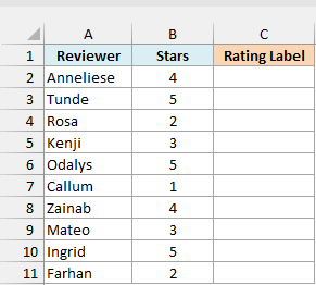
Here is the formula:

=CHOOSE(B2:B11,"Very Poor","Poor","Average","Good","Excellent")

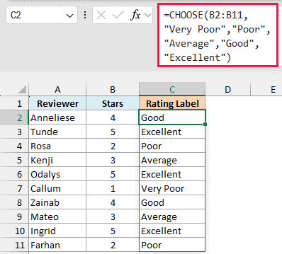
The formula lists five labels in rating order, so a 1 returns “Very Poor” and a 5 returns “Excellent”.

The labels are text, so each one goes in double quotes inside the formula.

Giving CHOOSE the whole range B2:B11 instead of one cell returns a label for every rating, so the labels spill into C2:C11.

If you are using Excel 2019 or earlier, enter the below formula in cell C2 and then copy it down the range:

=CHOOSE(B2,"Very Poor","Poor","Average","Good","Excellent")

If a cell in C2:C11 already has something in it, the formula can’t spill and shows a #SPILL! error. Clear the cells blocking it, and the labels appear.

If your ratings are in an Excel Table, put the formula in a column outside the table because spilling formulas don’t work inside a table.

A rating like 4.5 has its decimal dropped, so CHOOSE returns “Good” instead of an error. That’s easy to miss.

Important: A 0, a blank cell, or a 6 returns #VALUE! because there’s no choice at that position. The IFERROR function can show a friendly message instead.

Example 2: Return Custom Labels for Weekdays

Now let’s pair CHOOSE with the WEEKDAY function to give each date a custom label.

Below is a family dinner plan with dates in column A, and I want to use each date’s day of the week to assign a dinner theme in column B.

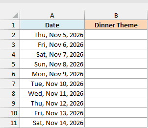
Here is the formula:

=CHOOSE(WEEKDAY(A2:A11,2),"Meatless Monday","Taco Tuesday","Pasta Night","Stir-Fry Night","Pizza Friday","Grill Night","Roast Dinner")

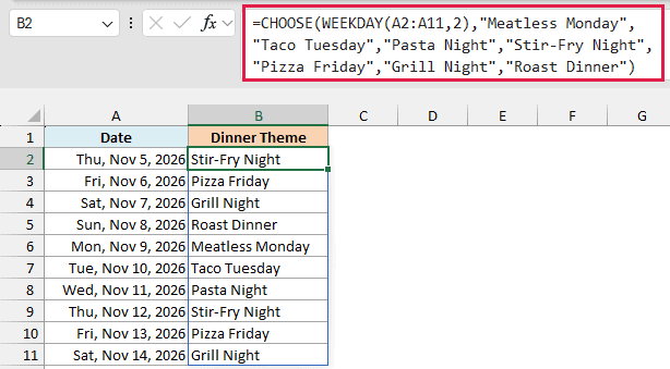
The themes spill into B2:B11. Thursday gets Stir-Fry Night, Friday gets Pizza Friday, and Saturday gets Grill Night.

Here is how this formula works:

• The WEEKDAY function returns a number for each date with WEEKDAY(A2:A11,2). Its second argument, 2, makes Monday return 1 and Sunday return 7.
• CHOOSE uses each number as a position in the theme list. That’s why the list starts with Meatless Monday and ends with Roast Dinner.

Pro Tip: If you only want day names like Monday, =TEXT(A2:A11,"dddd") does it without CHOOSE. Use CHOOSE for custom labels the TEXT function can’t produce.

A long list inside a formula is easy to get wrong when the themes change. If they change often, keep them in a small table and look them up instead.

Example 3: Find Fiscal Quarters from Dates

You can use the same idea to match months to fiscal quarters.

Below are office equipment purchases for a business whose fiscal year starts on April 1, and I want the fiscal quarter for each purchase date in column C.

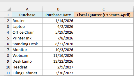
Here is the formula:

="Q"&CHOOSE(MONTH(B2:B11),4,4,4,1,1,1,2,2,2,3,3,3)

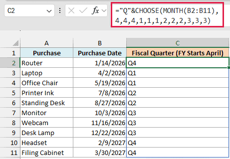
The quarter labels spill into C2:C11. The Router bought on January 14, 2026 gets Q4, while the Laptop bought on April 2, 2026 gets Q1.

Here is how this formula works:

• MONTH(B2:B11) returns a month number from 1 to 12 for each purchase date.
• CHOOSE matches that number to one of the 12 quarter numbers, written in January-to-December order.
• January through March map to 4, April through June to 1, July through September to 2, and October through December to 3.
• "Q"& adds the letter Q before each number, so the result reads Q1, Q2, Q3, or Q4.

To use a different fiscal start, reorder the 12 choices. For a July start, the list becomes 3,3,3,4,4,4,1,1,1,2,2,2.

For calendar quarters, see this guide to getting the quarter from a date.

Example 4: Pick a Calculation for Each Code

Your choices can be calculations too.

Below are ten parking garage tickets with vehicle classes and hours parked, and I want to calculate each ticket’s fee in column D.

The rate card shows class 1 as Motorbike at $3 flat, class 2 as Car at $2.50 per hour, and class 3 as Van at $4 + $3 per hour.

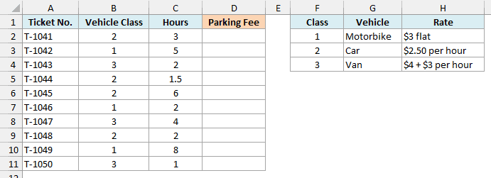
Here is the formula:

=CHOOSE(B2:B11,3,2.5*C2:C11,4+3*C2:C11)

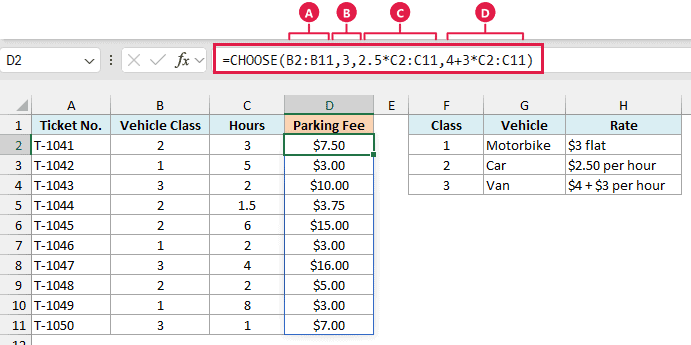
The fees spill into D2:D11, which is formatted as currency. Each vehicle class picks the result of a different calculation.

Here is how this formula works:

• (A) B2:B11 supplies the vehicle class codes, which select choice 1, 2, or 3 for each ticket.
• (B) Choice 1 is 3, so a motorbike costs $3.00 regardless of the hours.
• (C) Choice 2 is 2.5*C2:C11, so a car costs $2.50 multiplied by its hours.
• (D) Choice 3 is 4+3*C2:C11, so a van costs $4.00 plus $3.00 multiplied by its hours.

For ticket T-1043, the class is 3 and the hours are 2. CHOOSE returns the third calculation: 4+3*2, which gives $10.00 in D4.

The rate card is only there for reference. The rates are typed into the formula, so changing the card won’t change the fees.

If rates change often, put them in cells and point the formula at those cells, so you only have to update the rates in one place.

If the vehicle class were text, like “Car” picked from a drop-down list, the SWITCH function would be a better fit because it matches text directly.

Example 5: Pick Random Items from a List

Let’s use CHOOSE to make the lunch decision for a whole week.

Below is a team lunch planner for Monday through Friday, and I want to pick a random lunch for each weekday in column B.

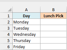
Here is the formula:

=CHOOSE(RANDARRAY(5,1,1,4,TRUE),"Pizza","Sushi","Tacos","Salad Bowl")

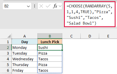
You get one random lunch in B2:B6 for each weekday. Your picks may differ from the screenshot, and the same lunch can appear more than once.

Here is how this formula works:

• RANDARRAY(5,1,1,4,TRUE) generates five rows and one column of random numbers. The minimum is 1, the maximum is 4, and TRUE makes them whole numbers.
• CHOOSE turns each number into the lunch in that position: Pizza, Sushi, Tacos, or Salad Bowl. The five results spill into B2:B6.

Important: The picks change on recalculation, such as an edit or F9. To keep them, copy B2:B6 and paste as values.

The RANDARRAY function is only in Excel 365, Excel 2021 and later, and Excel for the web.

If you’re using Excel 2019 or earlier, use the RANDBETWEEN function instead.

It returns one random number per cell, so enter the below formula in B2 and copy it down to B6:

=CHOOSE(RANDBETWEEN(1,4),"Pizza","Sushi","Tacos","Salad Bowl")

Example 6: VLOOKUP with CHOOSE to Look Left

Let’s finish with a trick you’ll see in older workbooks.

Below is a hotel guest list, and I want to find the guest for room 214 (entered in F1), with the result in F2.

The list has ten guests, with room numbers to the right of the names. That’s a problem for the VLOOKUP function, because it can’t look left.

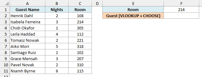
Here is the formula:

=VLOOKUP(F1,CHOOSE({1,2},C2:C11,A2:A11),2,FALSE)

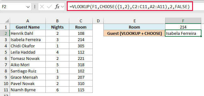
This returns Isabela Ferreira in F2. CHOOSE makes it work by putting the Room column first inside the formula, with Guest Name beside it.

Here is how this formula works:

• CHOOSE({1,2},C2:C11,A2:A11) uses the array constant {1,2} as index_num. It returns both choices side by side, building a two-column table in memory.
• Choice 1 is C2:C11, so Room becomes the first column. Choice 2 is A2:A11, so Guest Name becomes the second column.
• The VLOOKUP function searches that table’s first column for 214 from F1. The argument 2 returns the guest from column 2, and FALSE asks for an exact match.

This trick is worth knowing for older workbooks. For a new formula, the XLOOKUP function is a better choice than the VLOOKUP function.

Just make sure your Excel version and the people you share the file with have it.

In Excel 365 or Excel 2021 and later, enter this formula in F3 to get the same guest with the XLOOKUP function:

=XLOOKUP(F1,C2:C11,A2:A11)

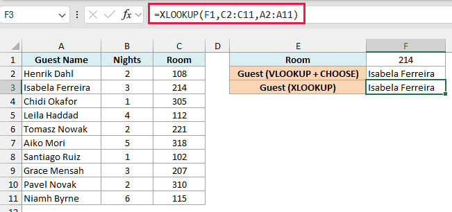
This also returns Isabela Ferreira. The XLOOKUP function looks left or right, so you can give it the room column and guest column directly.

If you’re using Excel 2019 or earlier, the INDEX and MATCH combination also looks left without rebuilding the table.

Enter the below formula in F3 instead:

=INDEX(A2:A11,MATCH(F1,C2:C11,0))

In this article, I showed you how to use CHOOSE to return labels, pick calculations and random items, and help VLOOKUP look left.

I hope you found this article helpful.

List of All Excel Functions

Other Excel Articles You May Also Like:

• VLOOKUP vs XLOOKUP Function – What’s the Difference?
• How to Generate Random Numbers in Excel
• VSTACK guide
• XMATCH
• Lookup the Second, the Third, or the Nth Value in Excel
• 20 Advanced Excel Functions and Formulas (for Excel Pros)