

If you want to pile separate ranges into one list in Excel, the VSTACK function is what you want.
VSTACK is a dynamic array function. It spills its results across the cells below, and to the right for multi-column data.
In this article, I’ll show you how to use VSTACK in Excel, from combining two lists to stacking sheets and filtering Excel Tables.
Follow along with the example file
VSTACK Function Examples.xlsx
Excel VSTACK Function Syntax
Here is the syntax of the VSTACK function:
=VSTACK(array1,[array2],...)
- array1 is the first range or array. It is required, and its rows sit at the top of the result.
- [array2], … are optional additional arrays. Each one goes below the one before it, in the exact order you list them.
Each argument tells the VSTACK function which data to stack. You can use a cell range, an Excel Table, or another formula’s result.
You can also type values as an array constant, or use a spilled range such as E2#. The # includes all the cells spilled from E2.
The result contains all the rows from your arrays, so its height is their total row count. The arrays don’t need the same number of rows.
The widest array sets the number of result columns. If another array is narrower, its extra columns show #N/A, as you’ll see in Example 3.
The columns line up by position, so matching header names won’t rearrange them. Keep the columns in the same order, as shown in Example 1.
The VSTACK function keeps the rows in their original order, including duplicates. Example 6 shows how to sort the combined list and remove repeats.
VSTACK is available in Excel for Microsoft 365 and Excel 2024, on Windows and Mac, and in Excel for the web.
It isn’t available in Excel 2021, 2019, or 2016. Those versions show #NAME? when you try a VSTACK formula.
For older versions, use Power Query to combine worksheets instead.
Power Query is also the better tool for combining many workbooks or very large datasets.
When to Use the VSTACK Function
Use VSTACK when you need to:
- Combine two or more lists or tables into a single range.
- Pull the same data layout from several sheets into one master list.
- Add your own header or extra rows to a list.
- Feed a combined range into SORT, UNIQUE, or FILTER.
- Keep a combined list that updates when the source values change.
HSTACK is its side-by-side twin. VSTACK adds rows below; HSTACK adds columns to the right.
Let me show you how this works with a few practical examples.
Example 1: Stack Two Lists into One
Let’s start with the simplest case.
Below I have two 5K sign-up lists with each runner’s name and age, and I want to combine them in columns G and H.
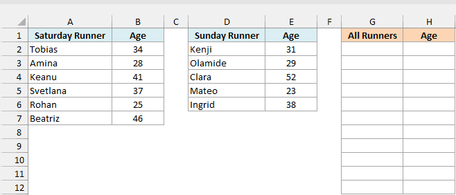
Here is the formula:
=VSTACK(A2:B7,D2:E6)
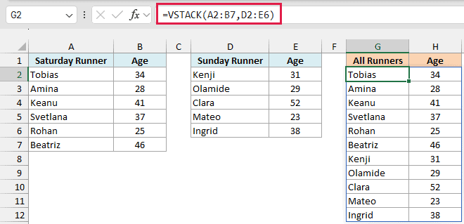
VSTACK takes the Saturday range first and drops the Sunday range right below it. Because you give it two columns, the name and age travel together.
The result spills into G2:H12, an 11-row list. The six Saturday runners, Tobias to Beatriz, come first, followed by the five Sunday runners, Kenji to Ingrid.
Notice you only type the formula once, in G2. Excel fills the rest of the range for you, and the result updates if a source name or age changes.
The order of the arguments is the order of the stack. Using =VSTACK(D2:E6,A2:B7) would put Sunday first.
Important: Keep the columns in the same order, name then age. If one list puts age first, VSTACK lines up the wrong values without giving an error.
Anything sitting in G2:H12 causes a #SPILL! error, so keep the result area clear and unmerged.
Example 2: Add Headers with an Array Constant
Sometimes your source lists don’t have the header you want on the final table.
Below are this month’s and next month’s movie watchlists, and I want one list with Movie and Runtime (min) headers in columns G and H.
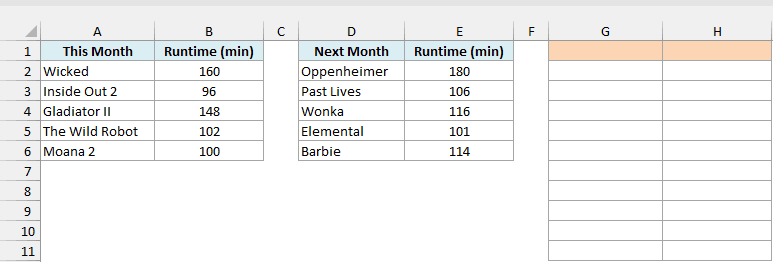
Here is the formula to enter in G1:
=VSTACK({"Movie","Runtime (min)"},A2:B6,D2:E6)
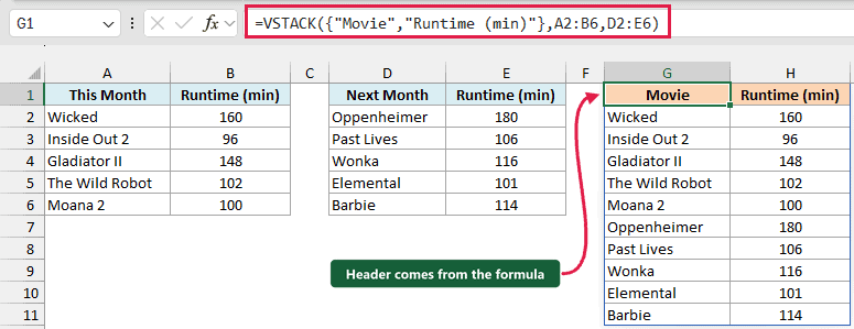
The {"Movie","Runtime (min)"} bit is an array constant. It’s a header row typed into the formula, with two columns separated by a comma.
VSTACK treats it like any other array and puts it first. Below it come the two movie ranges, so the header sits once at the top of the whole stack.
G1:H11 contains the header, the five This Month movies, and then the five Next Month movies. Wicked comes first and Barbie comes last.
There are three arguments here: the header array and two data ranges. You can keep adding more ranges the same way.
Example 3: Stack Ranges with Different Column Counts
When one range is narrower than another, you’ll see #N/A, and it helps to know why.
Below I have this month’s fixed bills and extra expenses, and I want to combine them in columns H to J.
The six bills have amounts and due dates, but the four extra expenses have no due date column.
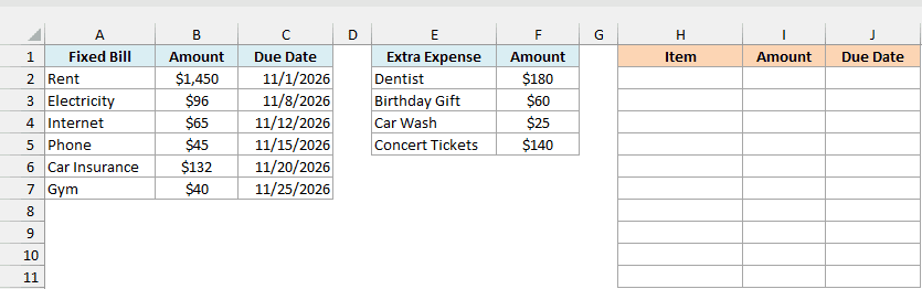
Here is the formula to enter in H2:
=VSTACK(A2:C7,E2:F5)
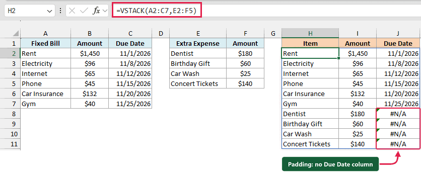
The wider range sets the result’s width at three columns. The six fixed bills come through with their amounts and due dates.
The four extra expenses have nothing for the third column, so VSTACK pads J8:J11 with #N/A. The data is fine; the second range simply has no due dates.
If you’d rather show blanks instead of the padding errors, wrap the stack in the IFNA function.
Enter this formula in L2:
=IFNA(VSTACK(A2:C7,E2:F5),"")
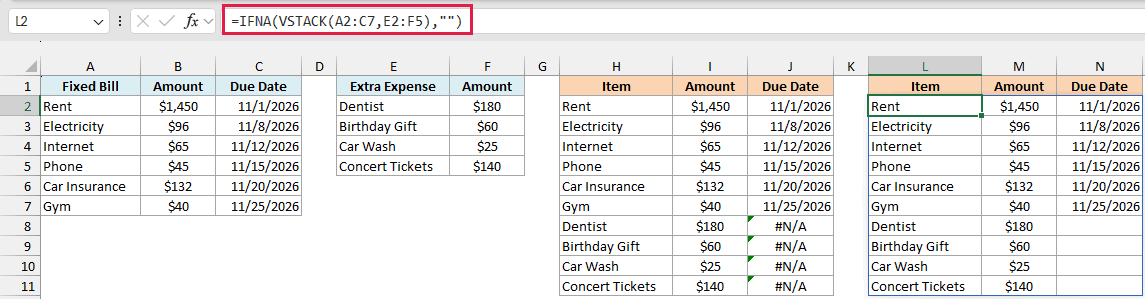
The same ten items spill into L2:N11. IFNA replaces #N/A with an empty string, so the four padding cells in N8:N11 look blank.
The IFNA function only replaces #N/A, so errors such as #DIV/0! or #REF! stay visible if they come from your source data.
The IFERROR function would hide those errors too, which is why the IFNA function is safer here.
Important: IFNA also hides genuine #N/A errors in your source. If you need to keep those visible, pad only the narrower range instead.
For that approach, use =VSTACK(A2:C7,EXPAND(E2:F5,,3,"")).
The EXPAND function adds a blank third column to the extra expenses before stacking, so genuine source #N/A errors stay visible.
VSTACK copies values, not cell formatting. Apply a date format to the Due Date columns in the results so the dates display correctly.
Example 4: Combine Two Sheets with VSTACK
You can also stack ranges that live on different worksheets.
A gym keeps new members on one sheet per branch, and below is the Downtown sheet with its five new members.
I want to combine it with the Harborside sheet into one roster on the Example 4 sheet, with the header just once.
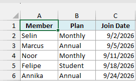
Below is the Harborside sheet with the same columns and four new members.
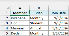
Here is the formula to enter in A1 to fill A1:C10, including the header row:
=VSTACK(Downtown!A1:C6,Harborside!A2:C5)
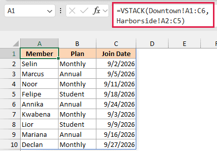
The Downtown range starts at row 1 so its header comes along. The Harborside range starts at row 2 so its header is left out.
That gives you one header at the top, followed by the five Downtown members and then the four Harborside members. Different row counts stack with no problem.
You can type the sheet references or click into each sheet while building the formula. The exclamation mark separates the sheet name from its cell range.
Apply a date format to the result’s Join Date column. VSTACK brings across the date values, but not their source formatting.
Pro Tip: Use Excel Tables instead of fixed ranges to pick up new rows automatically. Example 7 shows how to stack table references.
Example 5: VSTACK Multiple Sheets and Ignore Blanks
With several sheets laid out the same way, you can stack them using one sheet reference.
A pet grooming shop logs bookings on Week 1, Week 2, and Week 3, with four, five, and three bookings.
Below is the Week 2 sheet, and I want to combine all three weeks on the Example 5 sheet without a separate reference for each sheet.
The formula checks A2:C7 on every week’s sheet, leaving room for up to six bookings a week, so it picks up new bookings in those rows.
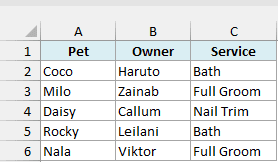
Here is the formula to enter in A2 for the stacked result in A2:C19:
=VSTACK('Week 1:Week 3'!A2:C7)
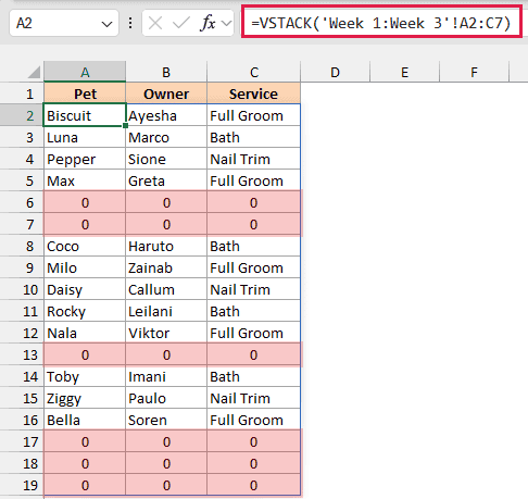
The 'Week 1:Week 3'!A2:C7 part is a 3D reference. It uses the same range on every sheet from Week 1 through Week 3, in tab order.
The formula stacks six rows from each sheet, so it returns 18 rows. Week 1 comes first, followed by Week 2 and Week 3.
Any sheet you drag between Week 1 and Week 3 joins the stack automatically. Moving a sheet outside those two tabs drops it from the reference.
Notice the rows displaying 0 in all three columns. These appear in rows 6, 7, 13, and 17 to 19.
Those source cells are empty. VSTACK displays them as 0, but they still count as empty in an ="" comparison. They aren’t cells containing a typed zero.
Let’s remove those blank rows by checking the Pet column for a name.
To remove the blank rows, enter this formula in E2:
=LET(all,VSTACK('Week 1:Week 3'!A2:C7),FILTER(all,CHOOSECOLS(all,1)<>""))
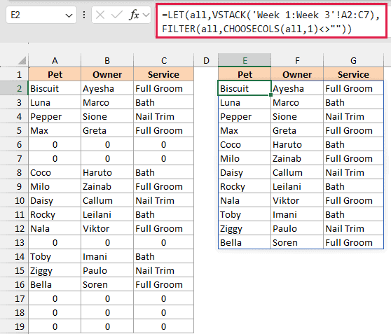
Now E2:G13 contains the 12 real bookings in order, starting with Biscuit and ending with Bella. The rows displaying zeros are gone.
Here is how this formula works:
- LET names the stacked block
all, so you only write the VSTACK and its 3D reference once. CHOOSECOLS(all,1)takes the first column of that block, which is the Pet column.<>""returns TRUE for rows with a pet name. The blank rows still count as empty here, even though the first result displays them as 0.- FILTER keeps the rows where that check returns TRUE and removes the rest.
For normal ranges in current Microsoft 365, trim references such as A2:.C7 remove trailing blanks in one go.
They don’t work with 3D references, so the FILTER function handles the blank rows in this example.
Example 6: Build a Sorted, Duplicate-Free List
VSTACK can also be the inner step of a bigger formula that sorts the combined list and removes repeats.
Below I have seven birthday guests and six picnic guests, and I want one alphabetized list without repeats in column E.
Eleni, Wren, and Lukas are on both lists.
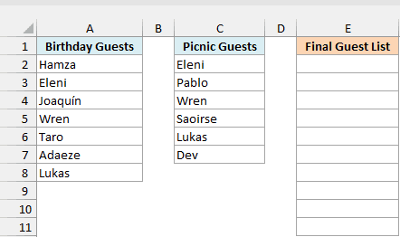
Here is the formula to enter in E2:
=SORT(UNIQUE(VSTACK(A2:A8,C2:C7)))
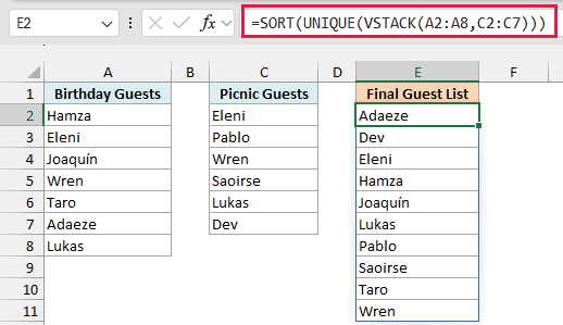
The ten names spill into E2:E11: Adaeze, Dev, Eleni, Hamza, Joaquín, Lukas, Pablo, Saoirse, Taro, and Wren.
Here is how this formula works:
VSTACK(A2:A8,C2:C7)first combines the two guest lists into one 13-name column.- UNIQUE removes the repeats, leaving ten names.
- SORT puts those names in A to Z order.
VSTACK itself never sorts or removes duplicates. That’s why UNIQUE and SORT wrap around it here.
If either source range had blank cells, they would appear as a 0 entry. Keep the ranges tight or use the FILTER cleanup from Example 5.
Example 7: Combine Excel Tables and Filter the Result
Let’s use table references for lists that will keep growing.
Below I have two mechanics’ bike repair jobs, and I want one list of bikes ready for pickup in columns I to K.
The tables are named LeoJobs (six jobs) and NadiaJobs (five), and both have Customer, Bike, and Status columns.
You can see or change a table’s name under Table Design > Table Name.

Here is the formula to enter in I2:
=FILTER(VSTACK(LeoJobs,NadiaJobs),VSTACK(LeoJobs[Status],NadiaJobs[Status])="Ready")
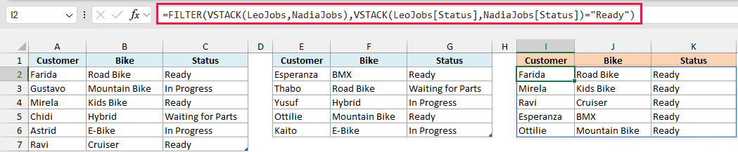
The result spills into I2:K6. It shows Farida’s Road Bike, Mirela’s Kids Bike, Ravi’s Cruiser, Esperanza’s BMX, and Ottilie’s Mountain Bike, all with Status Ready.
Here is how this formula works:
VSTACK(LeoJobs,NadiaJobs)stacks the two tables’ data rows. A table reference leaves out its header row.VSTACK(LeoJobs[Status],NadiaJobs[Status])stacks just the Status columns in the same order, so the two stacks line up row for row.="Ready"checks each status and returns TRUE or FALSE for that row.- FILTER keeps the rows where the check returns TRUE.
Because the sources are Tables, adding a new job to either table updates the combined list automatically. You don’t need to edit the formula’s ranges.
If no bikes are ready, the FILTER function has no rows to return, so it shows #CALC!.
To show a message instead, add "None ready" as the FILTER function’s third argument, after the ="Ready" test.
Important: Keep the formula outside both tables, as it is in I2. VSTACK and FILTER can’t spill inside an Excel Table, and doing so gives #SPILL!.
Stacking two separate FILTER results can fail with #CALC! as soon as one mechanic has no ready bikes. Stacking first lets FILTER check both lists together.
In this article, I showed you how to stack lists with VSTACK, add headers, and handle ranges with different column counts.
I also covered combining sheets and Excel Tables, removing blank rows, and sorting and filtering the stack.
I hope you found this article helpful.
Other Excel Articles You May Also Like:
