

The DDB function in Excel calculates how much an asset depreciates in a given period using the double declining balance method. It writes off more of the asset’s value in the early years and less as the asset gets older.
That suits things like vehicles, computers, and kitchen equipment, which lose most of their value soon after you buy them. You can also change the rate, so the same function handles a 150% declining balance or any other factor.
The examples below start with one year of depreciation for a single asset, then build full yearly and monthly schedules, handle a whole asset list with one formula, and track the book value to see where DDB falls short.
Follow along with the example file
DDB Function Examples.xlsx
DDB Function Syntax
Here is the syntax of the DDB function:
=DDB(cost, salvage, life, period, [factor])
- cost – the price you paid for the asset.
- salvage – the value of the asset at the end of its useful life. It can be 0.
- life – the number of periods over which the asset is depreciated (usually years).
- period – the period you want the depreciation for. It has to use the same unit as life.
- [factor] – optional. The rate at which the balance declines. If you leave it out, Excel uses 2, which is the double declining balance method.
The yearly rate is factor divided by life. So with the default factor of 2 and a 5-year life, DDB takes 40% of whatever value is left at the start of each year.
The salvage value doesn’t change that rate. DDB only uses it as a floor, so it never depreciates the asset below its salvage value.
The period has to be a number from 1 up to the life. A period of 0, or one bigger than the life, returns the #NUM! error.
You also get #NUM! if any of the arguments is a negative number.
If you type a comma after the period with nothing after it, like =DDB(1000,100,5,1,), Excel reads the factor as 0 and returns #NUM!. So when you want the default factor, leave it out completely.
The DDB function works in all Excel versions, including Excel 365, 2024, 2021, 2019, 2016, Mac, and the web.
When to Use the DDB Function
Use this function when you need to:
- Find the depreciation of an asset for a specific year
- Build a depreciation schedule for the full life of an asset
- Use a declining balance rate other than double, such as 150%
- Work out monthly depreciation instead of yearly
- Get this year’s depreciation for every asset in a list at once
Let me show you a few practical examples of how to use the DDB function.
Example 1: Calculate First-Year Depreciation with DDB
Let’s start with a simple example.
Below are the details of an espresso machine bought for a café, and I want to get its depreciation for year 1 in cell B8.
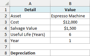
Here is the formula:
=DDB(B3,B4,B5,B6)
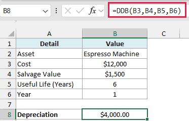
The formula returns $4,000. Since I left out the factor, DDB uses 2, so the rate is 2 divided by the 6-year life, which is about 33.33%.
In the first year, the full $12,000 cost is still on the books, so the depreciation is $12,000 x 33.33% = $4,000. Change the year in B6 to 2, and DDB applies the same rate to the $8,000 that’s left, which gives $2,666.67.
Example 2: Create a Double Declining Balance Depreciation Schedule
Now let’s get the depreciation for every year of an asset’s life with a single formula.
Below are the details of a delivery truck, with the years 1 to 8 listed in column A, and I want the depreciation for each year in column B.
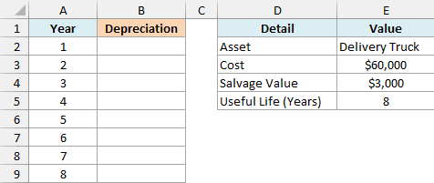
Here is the formula:
=DDB(E3,E4,E5,A2:A9)
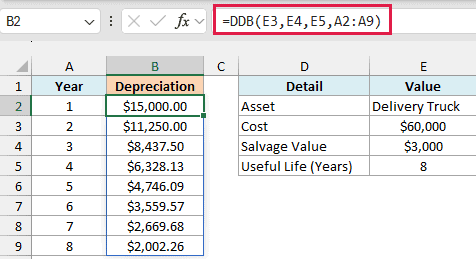
Since the period argument is the whole range A2:A9, DDB returns one result for each year, and the results spill down to B9. Year 1 is $15,000 (25% of the $60,000 cost), and every year after that takes 25% of a smaller remaining value.
That’s why the amounts drop each year, from $15,000 in year 1 to $2,002.26 in year 8. The truck loses most of its value in its first few years, which is exactly how the declining balance method is meant to work.
If you are using Excel 2019 or earlier, enter the below formula in cell B2 and then copy it down to B9:
=DDB($E$3,$E$4,$E$5,A2)
The dollar signs make the cost, salvage, and life cells absolute references, so only the year changes as you copy the formula down. Examples 3 and 4 work the same way.
Example 3: Use a Different Factor (150% Declining Balance)
Double declining balance is the default, but you can use any rate by changing the factor.
Below are the details of a pizza oven with a factor of 1.5 in cell E6, and I want a 150% declining balance schedule for its 7-year life in column B.
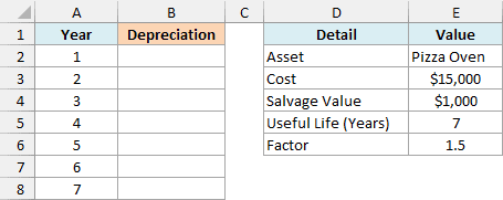
Here is the formula:
=DDB(E3,E4,E5,A2:A8,E6)
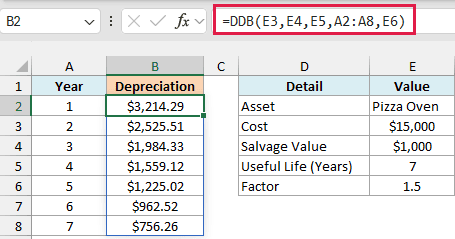
With a factor of 1.5, the rate is 1.5 divided by 7, which is about 21.43%. So year 1 is $3,214.29 instead of $4,285.71 with the default factor of 2, and the depreciation gets spread more evenly across the years.
Even a factor of 1 still gives you a declining balance, not straight-line depreciation. If you want the same amount every year, use the SLN function instead.
Since the factor is in its own cell, you can change it to 1.25 or 3 and the whole schedule updates.
Example 4: Calculate Monthly Depreciation
Some businesses track depreciation by month instead of by year, and DDB can do that too.
Below are the details of an office copier with a useful life of 4 years, and I want the depreciation for each of the first 12 months in column B.
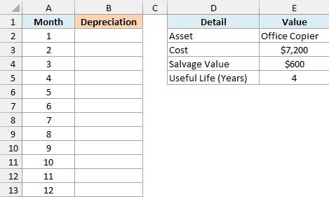
Here is the formula:
=DDB(E3,E4,E5*12,A2:A13)
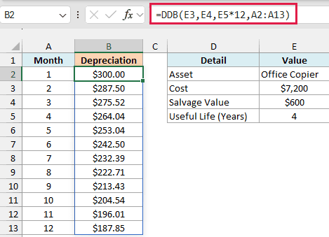
Here, E5*12 turns the 4-year life into 48 months, so the period values in A2:A13 count months instead of years. The monthly rate is 2 divided by 48, which makes month 1 equal to $7,200 x 2/48 = $300.
Important: If you keep the life in years and enter months as the period, DDB gives wrong results, and periods above 4 return #NUM!. Always convert the life to the same unit as the period.
The 12 monthly amounts add up to $2,879.52, which is less than the $3,600 that DDB gives for year 1 with a yearly life.
That’s because the declining balance is applied every month instead of once a year, so you can’t just divide the yearly number by 12.
Example 5: Get DDB Depreciation for Multiple Assets at Once
You can also pass ranges to all the arguments to get the depreciation for a whole asset list in one go.
Below is an asset list for a small business with the cost, salvage value, useful life, and the year each asset is in, and I want this year’s depreciation for every asset in column F.
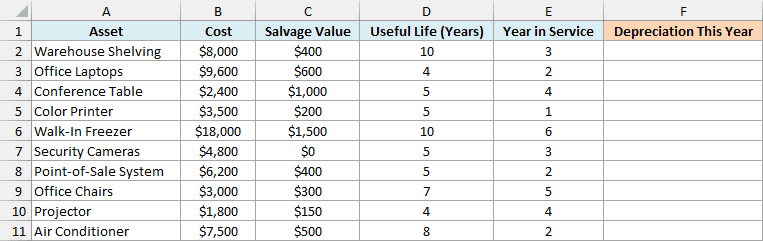
Here is the formula:
=DDB(B2:B11,C2:C11,D2:D11,E2:E11)
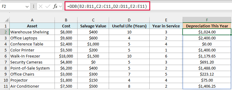
DDB pairs up the four ranges row by row, so each asset gets its own result using its own cost, salvage, life, and year. The results spill down to F11.
Look at the Conference Table, which returns $0. Its $1,000 salvage value is high compared to its $2,400 cost, so its remaining value reached $1,000 back in year 2, and DDB won’t depreciate it any further.
The Projector runs into the same floor. The normal 50% rate would give $112.50 in year 4, but that would take it below its $150 salvage value, so DDB returns only the $75 that’s left.
If you are using Excel 2019 or earlier, enter the below formula in cell F2 and then copy it down to F11:
=DDB(B2,C2,D2,E2)
Example 6: Track Book Value and Spot Where DDB Stops Short
Let’s step it up and see what the asset is worth at the end of each year.
Below is the DDB schedule for a forklift, and I want the book value (what the asset is still worth on the books) at the end of each year in column C.
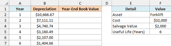
Column B already has the yearly depreciation from the formula =DDB(F3,F4,F5,A2:A7), which spills down to B7.
Here is the formula:
=F3-SCAN(0,B2#,LAMBDA(a,b,a+b))
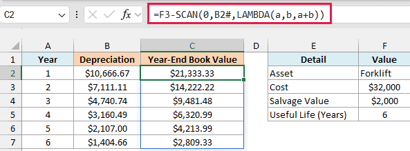
How this formula works:
- B2# refers to the whole spilled depreciation range that starts in B2.
- The SCAN function goes through that range and returns a running total, so you get the total depreciation up to the end of each year.
- The LAMBDA inside SCAN tells it how to build that total: add each year’s depreciation (b) to the total so far (a).
- Subtracting those running totals from the $32,000 cost in F3 gives the book value at the end of each year.
The SCAN function works only in Excel 365 and Excel 2024.
If you are using an older version, first fill column B with the copy-down DDB formula from Example 2 (pointing it at F3, F4, and F5), then enter the below formula in cell C2 and copy it down to C7:
=$F$3-SUM($B$2:B2)
Now look at the last row. After 6 years, the forklift is still on the books at $2,809.33, which is $809.33 more than its $2,000 salvage value.
This happens because DDB always takes a percentage of what’s left, so with a low salvage value, it can run out of years before reaching it. DDB stops at the salvage value, but it never adds a catch-up amount in the final year.
Important: DDB doesn’t always depreciate an asset all the way down to its salvage value. If you need the full amount written off by the end of the asset’s life, use the VDB function, which switches to straight-line depreciation once that gives a bigger amount.
For this forklift, the VDB function gives the same amounts as DDB for the first 4 years, then $2,160.49 in each of years 5 and 6. That brings the book value down to exactly $2,000.
So these are six practical ways to use the DDB function in Excel. It gives you the depreciation for one period or a whole schedule, works with a custom factor and with months, and handles a full asset list with one formula.
I hope you found this Excel tutorial useful.
Other Excel Articles You May Also Like:
