Creating Actual vs Target Chart in Excel (2 Examples)

If you work involves reporting the actual and target data, you may find it useful to present the actual values versus the target values in a chart in Excel.

For example, you can show the actual sales values versus the target sales values, or the satisfaction rating achieved versus the target rating.

There can be multiple ways to create a chart in Excel that shows the data with Actual Value and the Target Value.

Here are the two representations that I prefer:

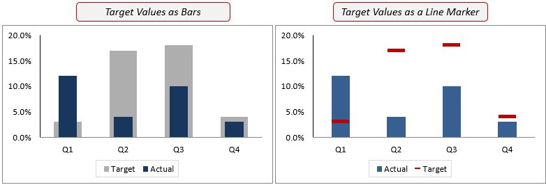
In the chart on the left, the target values are shown as the wide gray bar and achieved/actual values are shown as the narrow blue bar.

In the chart on the right, the actual values are shown as the blue bars and the target values are shown as red markers.

In this tutorial, I will show you how to create these two actual vs target charts.

Click here to download the example file.

#1 Actual vs Target Chart in Excel – Target Values as Bars

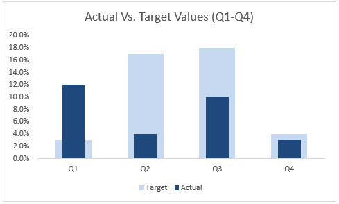
This chart (as shown below) uses a contrast in the Actual and Target bars to show the whether the target has been met or not.

It is better to have the Actual Values in dark shade as it instantly draws attention.

Here are the steps to create this Actual vs Target chart:

1. Select the data for target and actual values.
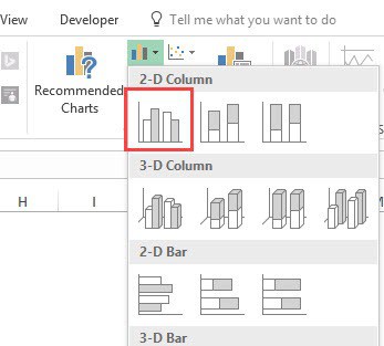
2. Go to the Insert tab.
3. In the Charts Group, click on the ‘Clustered Column Chart’ icon.
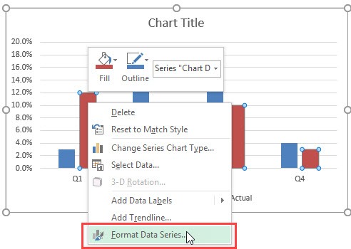
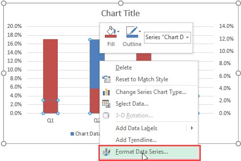
4. In the chart that is inserted in the worksheet, Click on any of the bars for Actual Value.
5. Right-click and select Format Data Series
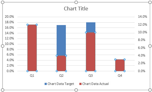
6. In the Format Series pane (a dialog box opens in Excel 2010 or prior versions), select ‘Secondary Axis in the Plot Series options.
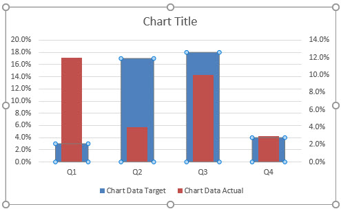
7. Your chart should now look somewhat as shown below.
8. Now, select any of the Target Value bars (simply click on the blue color bar), right-click and select ‘Format Data Series’.
9. In the ‘Format Data Series’ pane (or dialog box if you’re using Excel 2010 or prior versions), lower the Gap Width value (I changed it to 100%). The idea is to increase the width of the bars to make it wider than normal.
   
10. Your chart should look as shown below.
11. (Optional Step) Select any of the Actual Value bars. Right-click and select Format Data Series. Make the gap width value 200%. This will reduce the width of the actual value bars.
12. Click on the secondary axis values on the right of the chart and hit the Delete key.
13. Now your chart is ready. Format the chart. Shade the Target values bar in a light color to get a contrast.

Here is what you will get as the final output.

Now let’s see another way to represent the same data in a chart.

Try it Yourself.. Download the File

#2 Actual vs Target Chart in Excel – Target Values as Marker Lines

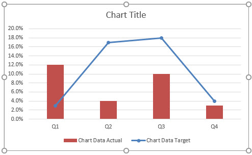
This chart (as shown below), uses marker lines to show the target value. The actual values are shown as columns bars.

Here are the steps this create this Actual Vs. Target chart in Excel:

1. Select the entire data set.
2. Go to Insert the tab.
3. In the Charts Group, click on the ‘Clustered Column Chart’ icon.
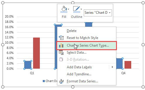
4. In the chart that is inserted in the worksheet, click on any of the bars for Target Value.
5. With the target bars selected, right-click and select ‘Change Series Chart Type’.
   
6. In Change Chart Type dialogue box, select Line Chart with Markers. This will change the target value bars into a line with markers.
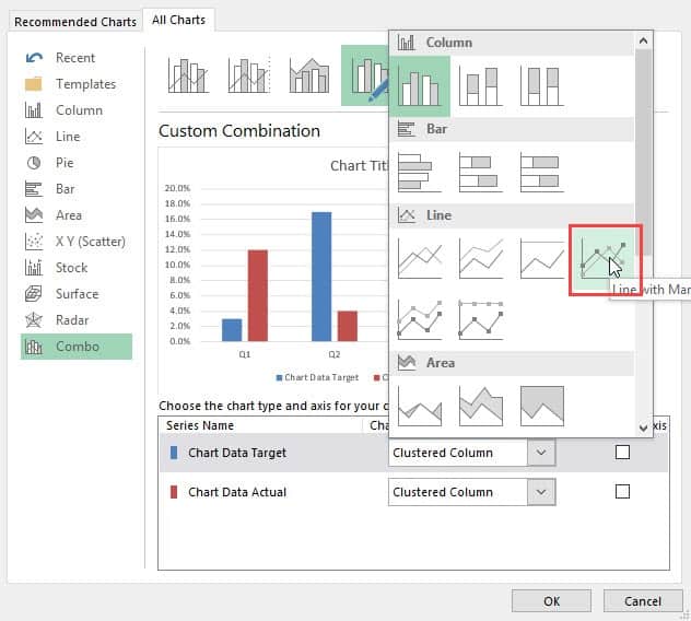
7. Click OK.
8. Your chart should look something as shown below.
9. Select the line, right-click and select Format Data Series.
10. In the Format Series pane, select ‘Fill & Line’ icon.
11. In the Line options, select ‘No Line’. This will remove the line in the chart and only the markers would remain.
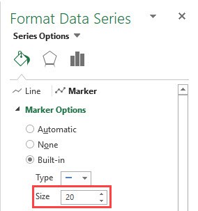
12. Select the ‘Marker’ icon. If you’re using an Excel version that shows a dialog box instead of the pane, you need to select ‘Marker Options’ in the dialog box.
13. In the Marker Options, select Built-in and select the marker that looks like a dash.
14. Change the size to 20. You can check what size looks best on your chart and adjust accordingly.

That’s it! Your chart is ready. Make sure you format the chart so that the marker and the bars are visible when there is an overlap.

Try it Yourself.. Download the File

These two charts covered in this tutorial are the ones that I prefer when I have to the show actual/achieved and target/planned values in an Excel chart.

If there are ways that you use, I would love to hear about it in the comments section.

You May Find the Following Excel Tutorials Useful:

• Creating a Dynamic Target Line in Excel Bar Charts.
• Creating a Step Chart in Excel.
• Creating a Milestone Chart in Excel.
• Creating a Gantt Chart in Excel.
• Creating a Heat Map in Excel.
• Creating a Histogram in Excel.
• Creating Combination Charts in Excel.
• Excel Sparklines – A Complete Guide.
• Advanced Excel Charts.