
Watch Video – Creating a Step Chart in Excel
A step chart can be useful when you want to show the changes that occur at irregular intervals. For example, the price rise in milk products, petrol, tax rate, interest rates, etc.
Let’s take the example of a Petrol hike in India. It can happen any day (as decided by the government) and the value remains constant between these changes. In such a case, a step chart is the right way to visualize such data points.
Unfortunately, Excel does not have an inbuilt feature to create a step chart, however, it can easily be created by rearranging the data set.
Step Chart in Excel
In this tutorial, you’ll learn:
- The difference between a Step Chart and a Line Chart.
- Creating a Step Chart using the “Line Chart technique”.
Line Chart Vs. Step Chart
A line chart would connect the data points in such a way that you see a trend. The focus in such charts is the trend and not the exact time of change.
On the contrary, a step chart shows the exact time of change in the data along with the trend. You can easily spot the time period where there was no change and can compare the magnitude of change in each instance.
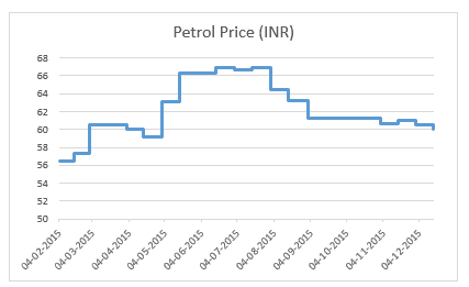
Here is an example of both the line chart and step chart – created using the same data set (petrol prices in India).
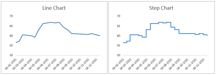
Both of these charts look similar, but the line chart is a bit misleading.
It gives you the impression that the petrol prices have gone up consistently during May 2015 and June 2015 (see image below).
But if you look at the step chart, you’ll notice that the price increase took place only on two occasions.
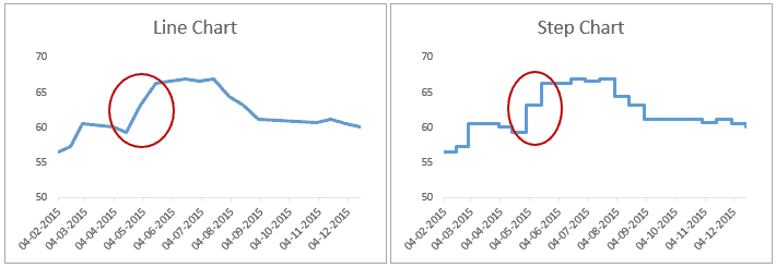
Similarly, a line chart shows a slight decline from September to November, while the step chart would tell you that this was the period of inactivity (see image below).

Hope I have established some benefits of using a Step Chart over a Line Chart. Now let’s go ahead a look at how to create a step chart in Excel.
Creating a Step Chart in Excel
First things first. The credit for this technique goes to Jon Peltier of PeltierTech.com. He is a charting wiz and you will find tons of awesome stuff on his website (including this technique). Do pay him a visit and say Hello.
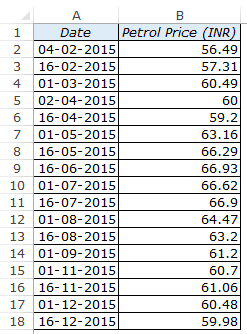
Here are the steps to create a step chart in Excel:
- Have the data in place. Here I have the data of petrol prices in India in 2015.
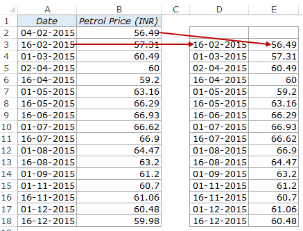
- Have a copy of the data arranged as shown below.
- The easiest way is to construct the additional data set right next to the original data set. Start from the second row of the data. In cell D3, enter the reference of the date in the same row (A3) in the original data set. In cell E3, enter the reference of the value in the row above (B2) in the original dataset. Drag the cells down to the last cell of the original data.
- Copy the original data (A2:B18 in the above example), and paste it right below the additional dataset that we created.
- You will have something as shown below (the data in yellow is the original data and green is the one that we created). Note that there is a blank row between the header and the data (as we started from the second row). If you are too finicky about how data looks, you can delete those cells.
- You don’t need to sort the data. Excel takes care of it.

- Select the entire data set, go to Insert –> Charts –> 2-D Line Chart.
- That’s it! You’ll have the step chart ready.
Download the Example File

How does this work:
To understand how this works, consider this – You have 2 data points, as shown below:

What happens when you plot these 2 data points on a line chart? You get a line as shown below:

Now to convert this line chart into a step chart, I need to show in the data that the value remained the same from 1 to 2 January, and then suddenly increased on 2 January. So I restructure the data as shown below:
I carry forward the data to the next date when the change in value happens. So for 2nd January, I have two values – 5 and 10. This gives me a step chart where the increase is shown as a vertical line.
The same logic is applied to the restructuring of the data while creating a full-blown step chart in Excel.
While it would be nice to get an inbuilt option to create step charts in Excel, once you get a hang of restructuring the data, it won’t take more than a few seconds to create this.
Download the Example File
Hope you find this useful. Let me know your thoughts/comments/suggestions in the comments below 🙂
Related Tutorials:
- Step Chart Tutorial by Jon Peltier.
- Line Chart Vs. Step Chart by Jon Peltier.
- Creating Actual Vs Target Charts in Excel.
Other Excel Charting Tutorials You Might Like:


How do you create a step chart when the label is not a date, but a value?
Direct and to the point. Many thanks!
Thanks for sharing! Is there a way to end the chart with a vertical line rather than a horizontal?
Thank you for the tutorial. Is it possible to have the axis not as date Format but only in Numbers like Step 1, Step 2, Step 3, …?
Dear Sir, I have a problem while sorting the same thing in various cell and to add their values. Can you please solve this problem for me. If you will give me your mail Id it would be better for me to send the data to resolve.
Hej how to add a second step chart to the graphics above?
like the one here: http://www.factcheck.org/2016/02/trump-vs-clinton/
Hello Sumit,
Thank you for sharing this wonderful tutorial. However I have a problem with my data set. Unable to load the picture. But the problem is that when I follow the above steps, I get 2 points as “16-02-2015” on X axis at different locations and Y axis values mapped to it ,56.49 and 57.31. Same is the case with every X axis point which is duplicate. PLease help.
Can you share the data file so I can have a look?
what you have problem in charts
Hi Sumit.
I kinda get this and it’s cool so thank you. But I’m not clear on why you need to copy the original data twice, as in col. D (with the extra row) + E. Why couldn’t it just be done from one set of data – add the blank row and copy the date (from below) and the amount (from above). I know it doesn’t work (I’ve tried it – lol) but I just don’t get the premise behind the dual sets of data in D + E. Can you explain that a little bit, pls. Thanks, Brenda
Hello Brenda.. Here is the logic. Let’s say the value on Day 1 is 10 and the value on Day 2 is 20. If I plot it in a line graph, I will have a line connecting 10 and 20. But If I have 3 values (Day 1 – 10, Day 2 – 10, Day 2 – 20), then it would show that from day 1 to day 2 the value was 10, and then on day 2 it went up to 20. The reason we duplicate values is so that we have this transition where day 1 to day 2 the value remains the same, and on day 2, it witnesses the change.
I also explain the logic in the video. Have a look as it also shows the graph in action.
Hope this helps.
Thanks Sumit. I appreciate your time.
Thank you very much for this idea
Thanks for commenting Hossein.. Glad you liked it 🙂
I really really like this tutorial. Not only for the how-to but especially for the WHY.
Thanks for dropping by Oz.. Glad you liked the tutorial 🙂
Hi! thnaks for sharing. I got a question about date column. Is it possible to format like months? I’ve tried and it didn´t work. thanks!
Hi Dilma.. Try this – right click on the axis and select format axis. In the Axis Options, select Axis type as Date. Should work with monthly data as well