How to Group Dates in Pivot Tables in Excel (Years, Months, Weeks)

If you want to see your sales by month, quarter, or year in a Pivot Table, you don’t need to add any helper columns to your data.

You can group the dates right inside the Pivot Table. It helps you analyze data by getting different views by dates, weeks, months, quarters, and years.

In this tutorial, I’ll show you how to group dates in a Pivot Table, fix the error you may get while doing it, and ungroup the dates when you’re done.

How to Group Dates in Pivot Tables in Excel

Before we start grouping, let’s have a look at the data we’ll be working with.

Suppose you have a dataset as shown below:

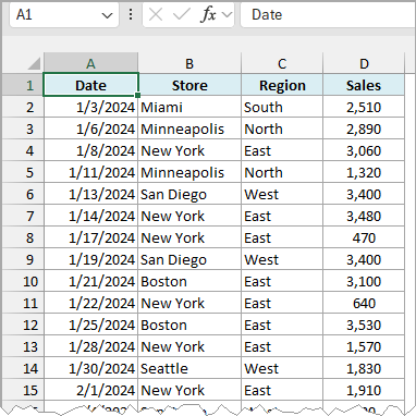
It has sales data by Date, Store, and Region (East, West, North, and South). The data spans across 374 rows and 4 columns, with dates from January 2024 to December 2025.

When you add the Date field to the Rows area in Excel 2016 or later, Excel groups the dates on its own. You’ll see years (with a plus icon to expand them) instead of individual dates.

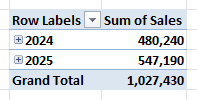
This is called automatic date grouping. It’s handy, but it doesn’t always give you the grouping you want.

If you press Control + Z right after adding the Date field, Excel undoes the grouping and shows every date instead. Here is what that looks like:

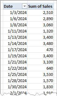
This Pivot Table summarizes sales data by date, but it isn’t quite helpful as it shows all the 300+ dates.

In such a case, it would be better to have the dates grouped by years, quarters, and/or months.

Whichever of these two you start with, the grouping steps below work the same way.

If you never want Excel to group dates automatically, you can turn off automatic date grouping completely.

Group Dates by Year in a Pivot Table

Let’s start with the simplest grouping, by years.

We’ll use the same sales data, which has dates for two years (2024 and 2025). Here is the Pivot Table with Date in the Rows area and Sum of Sales in the Values area:

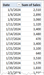
Here are the steps to group these dates by years:

1. Right-click on any date in the Pivot Table and click on Group. You can also go to the PivotTable Analyze tab (called Analyze in older versions) and click on Group Field.

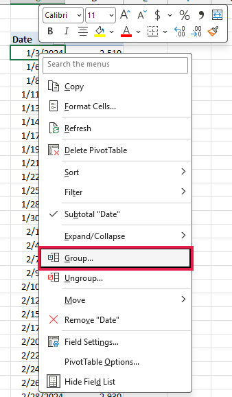
2. In the Grouping dialog box, select Years. You can select more than one option by simply clicking on it, and clicking a selected option deselects it. By default, Months is already selected, so click on Months to deselect it.

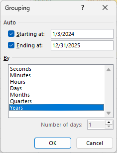
It picks the ‘Starting at’ date and ‘Ending at’ date based on the source data. If you want, you can change these.

3. Click OK.

This would summarize the Pivot Table by years.

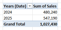
Note: I am using the tabular form layout in the above snapshot.

This summarization by years is useful when you have many years of data. In this case, with only two years, it would be better to have the quarterly or monthly data.

Pro Tip: You can also select any date and press Alt + Shift + Right Arrow to open the Grouping dialog box. Here are more Pivot Table shortcuts.

If you get a “Cannot group that selection” message, one of the dates in your data isn’t a real date. Here’s how to fix it.

Group Dates by Quarter (and Year) in a Pivot Table

In the above dataset, it makes more sense to drill down to quarters or months to have a better understanding of the sales.

Here is the same Pivot Table, with Date in the Rows area and Sum of Sales in the Values area:

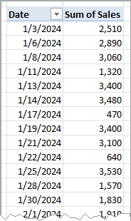
Here is how you can group these by quarters:

1. Right-click on any date in the Pivot Table and click on Group.

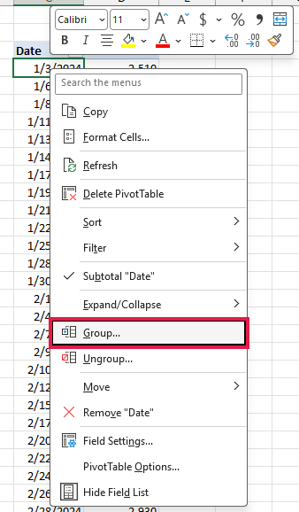
2. In the Grouping dialog box, select Quarters and deselect any other selected option(s).

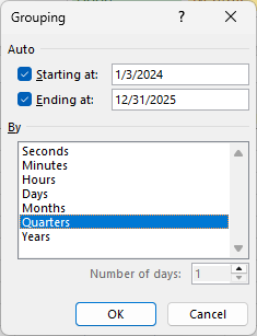
3. Click OK.

This would summarize the Pivot Table by quarters.

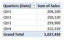
The issue with this Pivot Table is that it combines the quarterly sales value for 2024 as well as 2025.

For example, Qtr1 shows 204,100, which is the sum of Quarter 1 sales in 2024 and 2025.

In a real-life scenario, you are most likely to analyze these quarters for each year separately. To do this:

1. Right-click on any quarter in the Pivot Table and click on Group.

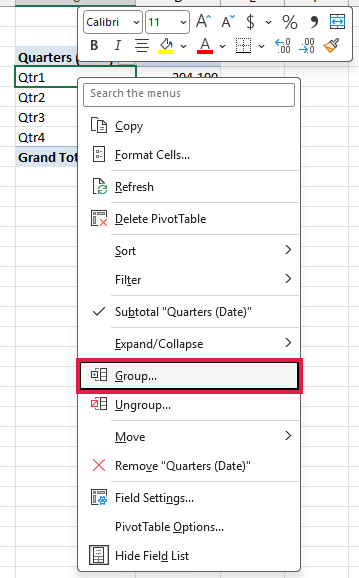
2. In the Grouping dialog box, select Quarters as well as Years.

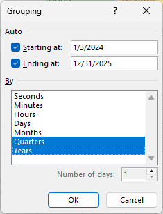
3. Click OK.

This would summarize the data by years and then, within years, by quarters. Something as shown below:

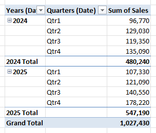
When you group dates by more than one time period, something interesting happens.

If you look at the field list, you’ll notice new fields have been added. In this case, they are Quarters (Date) and Years (Date).

Note that these new fields are not a part of the data source.

They are created in the Pivot Cache to quickly group and summarize data. When you ungroup the data, these fields will vanish.

Important: Since the grouping lives in the Pivot Cache, grouping dates in one Pivot Table also groups them in every other Pivot Table that shares the same cache.

The benefit of having these new fields is that now you can analyze the data with quarters in rows and years in columns.

All you need to do is drag the Years (Date) field from the Rows area to the Columns area.

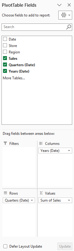
And here is the result, with years side by side:

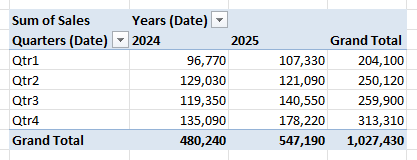
Now it’s easy to compare each quarter across the two years. For example, Qtr4 went up from 135,090 in 2024 to 178,220 in 2025.

Group Dates by Month and Year in a Pivot Table

Similar to the way we grouped the data by quarters, we can also do this by months. For example, if you have credit card data, you may want to see your spending month by month.

We’ll again use the sales data. Here is the Pivot Table with Date in the Rows area and Sum of Sales in the Values area:

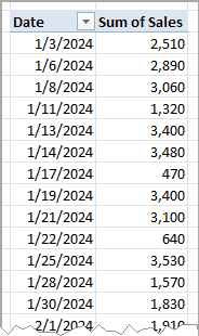
It is advisable to use both Years and Months to group the data instead of only using months (unless you only have data for one year or less).

Otherwise, January of both years gets added together, just like the quarters did above.

Here are the steps to do this:

1. Right-click on any date in the Pivot Table and click on Group.

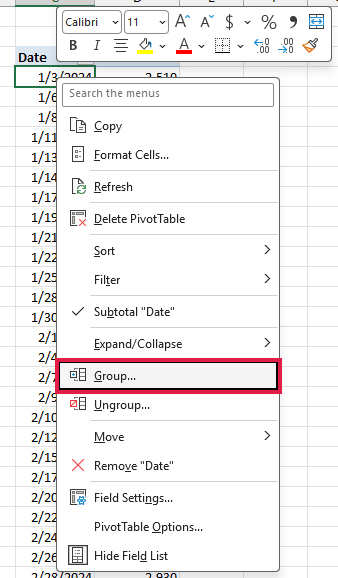
2. In the Grouping dialog box, select Months as well as Years.

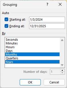
3. Click OK.

This would group the date field and summarize the data as shown below:

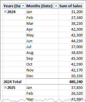
Again, this adds new fields (Months (Date) and Years (Date)) to the PivotTable Fields list.

You can simply drag it to the Columns area to get the years in columns and the months in rows. You will get something as shown below:

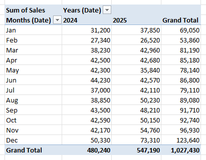
December is the biggest month in both years here, with 50,330 in 2024 and 73,310 in 2025.

Group Dates by Week in a Pivot Table

While analyzing data such as store sales or website traffic, it makes sense to analyze it on a weekly basis.

When working with dates in Pivot Tables, grouping dates by week is a bit different than grouping by months, quarters, or years.

There is no inbuilt option to group by weeks, so you group by days and specify the number of days to be used while grouping.

We’ll use the same sales data. Here is the Pivot Table with Date in the Rows area and Sum of Sales in the Values area:

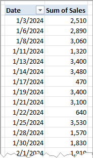
Here is how you can group dates by weeks:

1. Right-click on any date in the Pivot Table and click on Group.

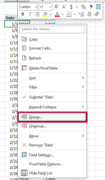
2. In the Grouping dialog box, select Days and deselect any other selected option(s). As soon as you do this, you would notice that the Number of days option (at the bottom right) becomes available.

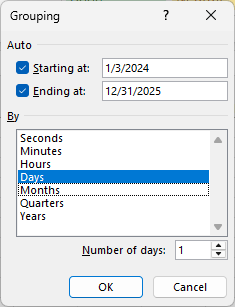
Note that for this to work, you need to select the Days option only.

3. In Number of days, enter 7 (or use the spin button to make the change).

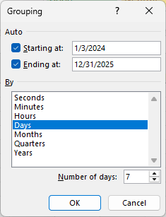
If you click OK at this point, your data would be grouped by weeks starting with January 3, 2024, which is a Wednesday. So the grouping would be from Wednesday to Tuesday every week.

To begin the week from Monday, you need to change the start date (by default, it picks the start date from the source data).

4. In the Starting at box, enter 1/1/2024, which is the Monday just before the first date in the data.

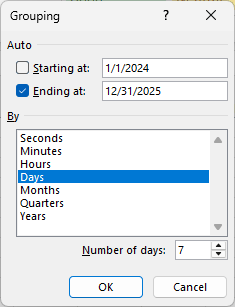
You could also start on January 8, 2024 (the next Monday).

But then the first few days of data go into a separate group labeled <1/8/2024, so starting a little before the data is the cleaner option.

5. Click OK.

This will group the dates by weeks as shown below:

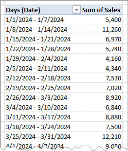
Each row is now one week, labeled with its start and end dates (such as 1/1/2024 – 1/7/2024). The header shows Days (Date) because, as far as Excel is concerned, you grouped by days.

The last group (12/29/2025 – 12/31/2025) is shorter than a week because that’s where the data ends.

Similarly, you can group dates by specifying any other number of days. For example, instead of weekly, you can group dates in a biweekly interval by entering 14.

Also note that when you group dates by a number of days, you can’t also group them by months, quarters, or years at the same time.

Important: Once any field in a Pivot Table is grouped (by days or any other way), you can’t add a calculated item to that Pivot Table. Calculated fields still work.

Group Dates by Hours, Minutes, or Seconds in a Pivot Table

If you are working with high volumes of data (such as call center data), you may want to group it by seconds, minutes, or hours.

You can use the same process to group the data by seconds, minutes, or hours.

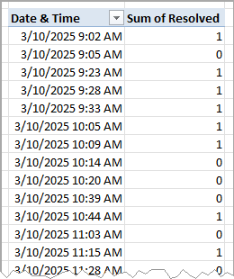
Suppose you have the call center data as shown below:

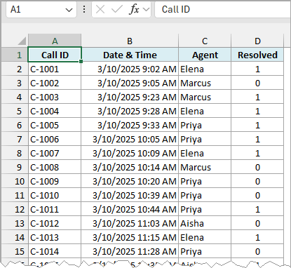
Each row is one call, with the date and time the call came in, the agent who handled it, and a 1 in the Resolved column if the call was resolved (0 if it wasn’t).

In this case, it may make sense for the call center manager to analyze how the number of resolved calls changes by the hour.

Here is how to group the data by hours:

1. Create a Pivot Table with Date & Time in the Rows area and Resolved in the Values area (it shows as Sum of Resolved).

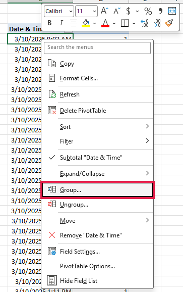
2. Right-click on any date in the Pivot Table and click on Group.

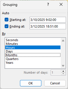
3. In the Grouping dialog box, select Hours and deselect any other selected option(s).

4. Click OK.

This will group the data by hours, and you will get something as shown below:

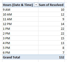
You can see that the row labels here are 9 AM, 10 AM, and so on, which are the hours in a day.

Using this Pivot Table, you can easily identify that most calls are resolved between 1 PM and 3 PM (22 in each of those two hours).

Note that grouping by hours only adds up the same hour across all three days. If you want to see each day separately, select Days as well as Hours in the Grouping dialog box.

Similarly, you can also group the dates by seconds and minutes.

Fix the Cannot Group That Selection Error

Sometimes, when you try to group dates, Excel shows a message that says “Cannot group that selection”.

This happens when at least one value in the date column of your source data is not a real date.

Most often, it’s a date that is stored as text (which often happens with data imported from other systems).

Here is a small dataset where this is the case:

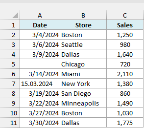
Notice that the date in cell A7 (15.03.2024) is aligned to the left, while all the other dates are aligned to the right.

That’s a quick way to spot a date stored as text, as Excel aligns real dates to the right by default.

If you create a Pivot Table from this data and try to group the dates, you get this error:

Here is how to fix it:

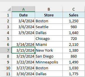
1. Replace the text date with a real date. In this example, select cell A7 and type 3/15/2024.

If you have a lot of such dates, fixing them one by one isn’t practical. You can convert text to dates in one go instead.

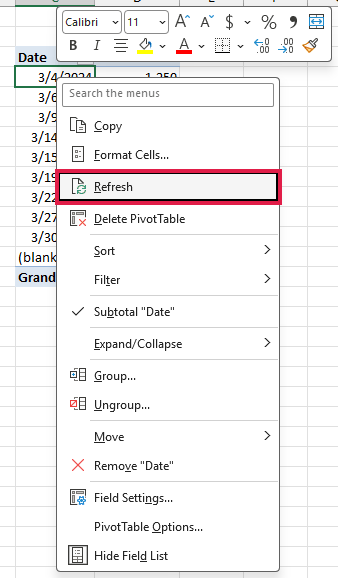
2. Right-click anywhere in the Pivot Table and click on Refresh.

3. Group the dates as shown in the sections above.

This dataset also has a blank date in cell A5. A blank date doesn’t stop the grouping, but it doesn’t disappear either.

Excel puts it in a separate group that is labeled with a less-than sign and the first date (<3/4/2024 in this example). So if you see such a row, check your data for blank dates.

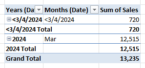
To fix this, enter the missing date (or remove the row if it shouldn’t be there), and then refresh the Pivot Table.

How to Ungroup Dates in a Pivot Table in Excel

If you want to go back to seeing the individual dates, you can ungroup them.

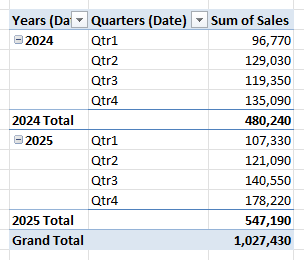
Here is a Pivot Table where the dates are grouped by years and quarters:

To ungroup dates in Pivot Tables:

1. Right-click on any of the grouped date cells in the Pivot Table and click on Ungroup. You can also go to the PivotTable Analyze tab and click on Ungroup.

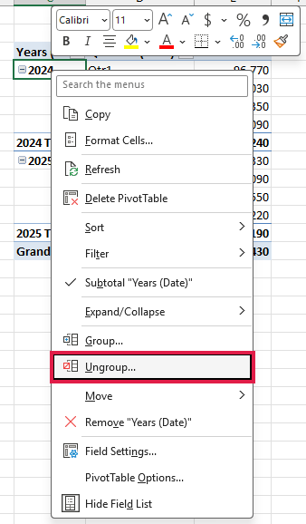
This would instantly ungroup any grouping that you have done, and the extra fields (such as Years (Date)) disappear from the field list.

Turn Off Automatic Date Grouping in Pivot Tables

As we saw at the start of this article, Excel 2016 and later versions group dates automatically when you add a date field to a Pivot Table.

If you’d rather see the individual dates every time (and group them yourself only when you need to), you can turn this off.

Here are the steps:

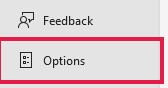
1. Click the File tab, and then click on Options.

2. In the Excel Options dialog box, click on Data in the left pane.

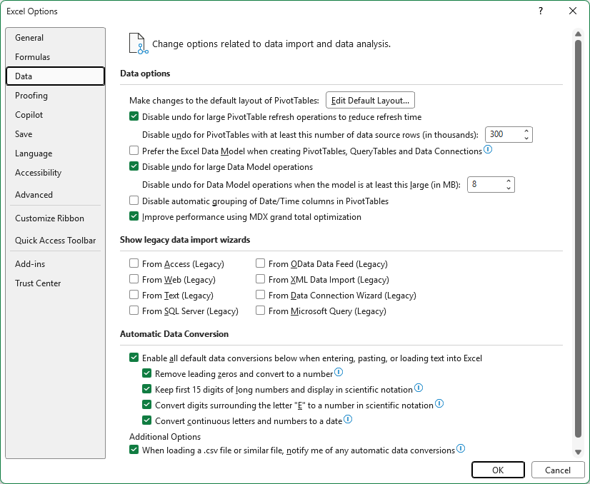
3. Check the option Disable automatic grouping of Date/Time columns in PivotTables.

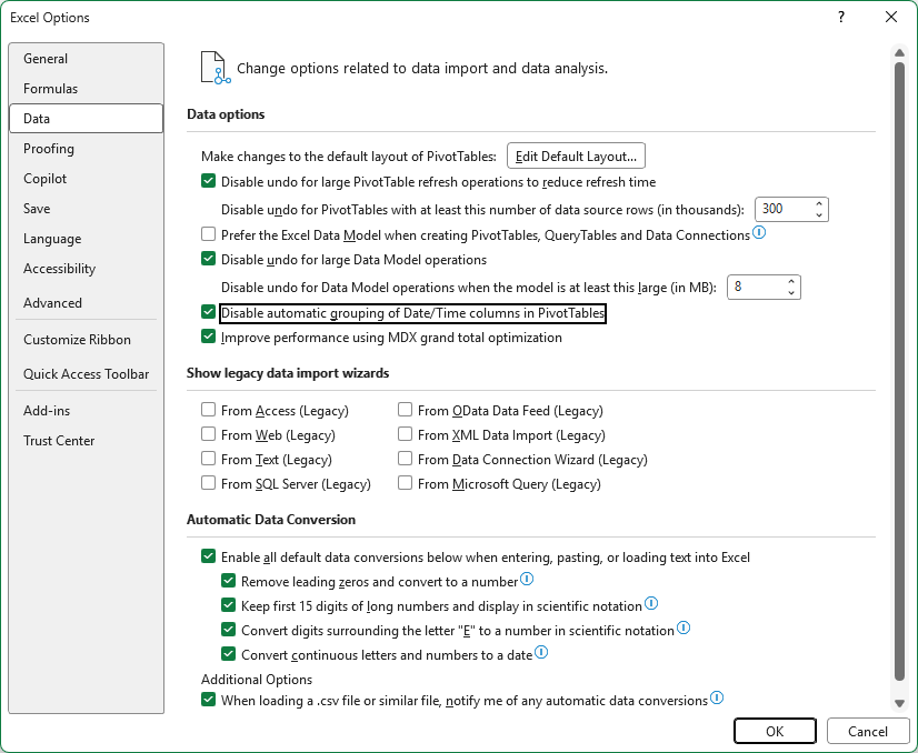
4. Click OK.

This is an Excel-wide setting, so it applies to all your workbooks, not just the current one. It also doesn’t change Pivot Tables that are already grouped.

This option is available in Excel 2019 and later versions (including Microsoft 365). In Excel 2016, press Control + Z right after adding the date field instead.

So these are the ways you can group dates in a Pivot Table in Excel, by years, quarters, months, weeks, and even hours.

I hope you found this tutorial useful.

Other Pivot Table Tutorials You May Like:

• Creating a Pivot Table in Excel: A Step by Step Tutorial.
• Preparing Source Data For Pivot Table.
• How to Group Numbers in Pivot Table in Excel.
• How to Filter Data in a Pivot Table in Excel.
• How to Apply Conditional Formatting in a Pivot Table in Excel.
• How to Refresh Pivot Table in Excel.
• How to Add and Use an Excel Pivot Table Calculated Field.
• Using Slicers in Excel Pivot Table.
• How to Replace Blank Cells with Zeros in Excel Pivot Tables.
• Count Distinct Values in Pivot Table
• Sort Pivot Table in Excel
• Pivot Table Limitations in Excel
• Sort Dates By Month in Excel