
A lot of people use dates in Excel for planning and keeping track of tasks and activities.
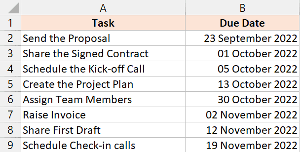
For example, below I have a data set where I have the tasks in column A and their due dates in column B.
It would be useful if there was a way to automatically highlight dates before today, so that I can visually see the tasks for which the due date has already passed.
Thanks to the awesome Conditional Formatting feature in Excel, you can easily highlight dates before today (i.e., the current date).
Let’s see a couple of ways to do this.
Note that I’m writing this article on 11 Oct, so that’s the date that would be used to highlight the cells with dates older than today.
Highlight Dates Before Today Using Quick Analysis Tool
Below I have a data set where I have the tasks in column A and their due dates in column B, and I want to highlight those dates there are before today.
And here are steps to highlight the cells with dates older than today:
- Select the cells that have the dates
- Click on the Quick Analysis Tool icon that shows up at the bottom right part of the selection
- Within the Formatting options, click on ‘Less than’. This will open the ‘Less Than’ dialog box

- Enter the below formula in the field in the ‘Less than’ dialog box
=TODAY()

- From the drop-down, select the formatting that you want to apply to the cells that have the dates before today. I will go with the default ‘Light Red Fill with Dark Red Text’

- Click OK
The above steps would highlight all the cells that have dates that are before today’s date.

Note that this would not highlight the cell if it has today’s date. This is because in the formula, we’ve asked Conditional Formatting to highlight all the cells with dates before today (and not including today).
If you would like today’s date to be highlighted as well, use =TODAY()+1 in step 4
A few important things to know:
- Excel picks up the current date from your system’s date and time settings. in case you change the date in your system, it would also impact the TODAY formula
- Conditional formatting is dynamic and would automatically update in case the dates in your original data set change. Also, whenever you open your Excel file, the TODAY function would refresh and take the value of the current date. This also means that your conditional formatting in the cells would accordingly update (so there could be dates that were not highlighted earlier, but are highlighted now as the current date has changed)
Also read: How to Remove Time from Date/Timestamp in Excel (4 Easy Ways)
Highlight Dates Before Today Using Conditional Formatting
In the above method, while I used conditional formatting for highlighting the cells with dates before today, I accessed conditional formatting using the Quick Analysis Tool.
In this section, I will show you how to access conditional formatting from the Home tab.
With this method, you get more options and a lot more control over how you want to highlight the cells.
For example, you can choose to highlight only the cells that contain the date or highlight the entire row (which you cannot do using the Quick Analysis Tool)
Highlighting Only the Cells with Dates
Below I have a data set where I have due dates in column B, and I want to highlight dates there are older than today.
Here are the steps to do this:
- Select the cells that have the dates
- Click the Home tab

- In The Styles group, click on ‘Conditional Formatting’
- Go to the ‘Highlight Cell Rules’ option
- In the options that show up, click on ‘Less than’. This will open the Less than dialog box

- Enter the below formula in the field
=TODAY()
- From the drop-down on the right, select the format in which you want to highlight the cells. If you don’t like the already specified options, you can click on the Custom Format option to get more formatting options. I will go with the default ‘Light Red Fill with Dark Red Text’ option
- Click Ok
The above steps would use conditional formatting to highlight cells that contain dates that are older than the current date.
Highlighting the Entire Row
So far, I have shown you how to highlight the cells that contain the date.
But what if you don’t want to just highlight the cell with the date, and instead highlight the entire row?
This can also be done easily with conditional formatting, but the steps would be slightly different.
Below I have a data set where I have the dates in column B, and I want to highlight the entire row wherever the date is before today’s date.
Here are the steps to do this:
- Select the entire dataset (A2:B9 in this example)
- Click the Home tab
- In the styles group, click on the Conditional Formatting option
- In the options that show up in the drop-down, click on the ‘New Rule’ option. This will open the ‘New Formatting Rule’ dialog box

- Select the option ‘Use formula to determine which cells to format’

- In the Formula field, enter the below formula
=$B2<TODAY()

- Click the Format button. This will open the Format Cells dialog box

- Select the ‘Fill’ tab and select the color with which you want to highlight the cell. I will go with the yellow color

- Click Ok
The above steps would highlight the rows wherever the date is before today’s date.

Let me quickly explain how this works.
Conditional formatting allows me to use a formula (that must return a True or a False) to analyze the selected cells.
In this example, I selected the entire data set (A2:B9), and then use the formula =$B2<TODAY() to analyze each cell.
Since I have used $B2 in the formula, it makes sure that when I am analyzing any cell in row 2, it would always use B2 as the cell in the formula.
So when it is analyzing cell A2, it uses the formula =$B2<TODAY(). If this formula returns a TRUE, the cell would be highlighted, else it would not be highlighted. And the same formula is used when it’s analyzing cell B2.
Now when it moves to the next row, and it needs to analyze cell A3, it uses the formula =$B3<TODAY(), and the same formula is used to analyze cell B3.
And so on.
By adding a dollar sign before the B in cell reference B2, I have made sure that for the entire row, the same formula is used.
Hence, If the date in column B is less than today’s date, the entire row gets highlighted.
Also read: How to Calculate Days Between Dates in Excel
Highlight Dates Within 30 or 60 or 90 Days Before Today
Sometimes, there is a need to highlight cells where the date is older than today but not older than 30 or 60, or 90 days.
This means that I want to highlight only those dates that are between today and 30 days before today.
This could be useful in case you have a list of tasks and you want to see which tasks have been completed in the last 30 days, or you have a list of invoices that have been paid and you want to see which invoices have been paid in the last 30 or 60 days.
Below I have a list of tasks along with their due dates in column B, and I want to highlight dates that are between today and 30 days ago.

Here are steps to do this:
- Select the cells that have the dates
- Click the Home tab
- Click on the Conditional Formatting icon
- Go to the Highlight Cell Rules option
- Click on the ‘Between’ option. This will open the Between dialog box

- In the first field, enter the below formula
=TODAY()-30

- In the second field enter the below formula
=TODAY()

- Select the format from the drop-down. I will go with the default ‘Light Red Fill with Dark Red Text’

- Click OK
The above should highlight all the cells that have dates that are between today and 30 days ago.

Note that this would also highlight the current date (today’s date). In case you want to exclude the current date from being highlighted, use =TODAY()-1 in step 7.
In this tutorial, I covered a couple of methods to highlight days before today using Conditional Formatting.
If you only want to highlight only the cells that contain the dates, you can do that using the Quick Analysis tool as well as the Conditional Formatting option in the ribbon.
I also covered how to highlight the entire row where the date in one column is before today’s date.
Other Excel articles you may also like:
- How to Calculate Years of Service in Excel
- How to Compare Dates in Excel (Greater/Less Than, Mismatches)
- Get Day Name from Date in Excel
- How to Add or Subtract Days to a Date in Excel (Shortcut + Formula)
- How to Highlight Weekend Dates in Excel?
- How to Autofill Only Weekday Dates in Excel (Formula)
- Calculate Time in Excel (Time Difference, Hours Worked, Add/ Subtract)


