

If you want all the text in your worksheet to stay visible, dragging every column and row by hand gets old quickly.
AutoFit can size them from their current contents, so you don’t have to guess the right width or height.
In this article, I’ll show you how to AutoFit columns and rows, what to do when AutoFit doesn’t work, and when to use Wrap Text or Shrink to Fit instead.
Follow along with the example file
AutoFit Excel Practice File.xlsx
What AutoFit Does in Excel
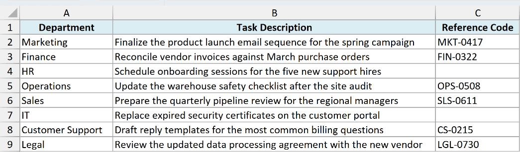
Below, I have a task list with Department, Task Description, and Reference Code columns. Some descriptions spill into the next empty cell, while others appear cut off.
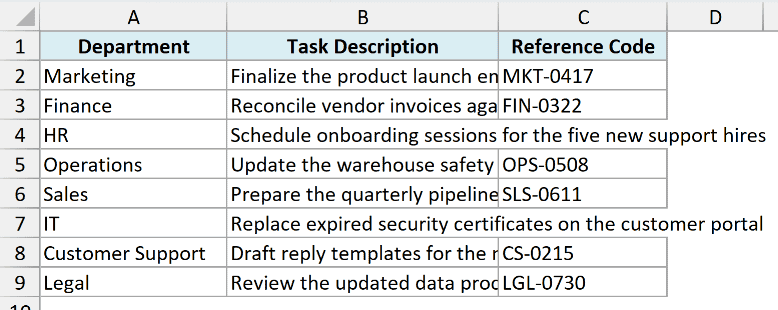
AutoFit expands or shrinks a column or row so its current contents fit.
- AutoFit Column Width changes a column’s width to fit its widest cell.
- AutoFit Row Height changes a row’s height to fit its tallest cell.
Excel often adjusts row height automatically when you enter multiple lines in a cell. However, an imported worksheet or a row with a fixed height may still need AutoFit Row Height.
You can also adjust the row height yourself when you need a specific size.
AutoFit sizes each selected column or row according to its own contents. It doesn’t make every cell the same size.
If you need a custom or uniform size instead, see How to Make Cells Bigger in Excel?
AutoFit a Column or Row With a Double-Click
The quickest way to AutoFit a column is to double-click its right border. This is the method I use most often because I find it the most convenient.
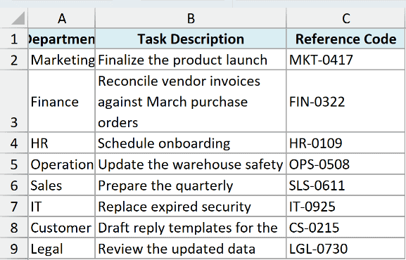
In this example, the task descriptions in column B are wider than the column. I want to fit the text to the cells without dragging the column boundary manually.
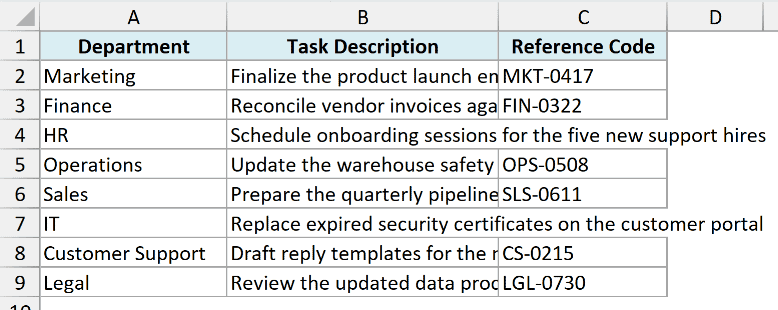
Here are the steps to AutoFit the column:
- Click the column B header to select the complete column.
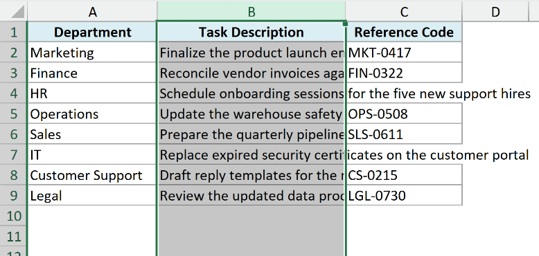
- Move the pointer to the right edge of the column B header. It will change to a two-sided arrow.
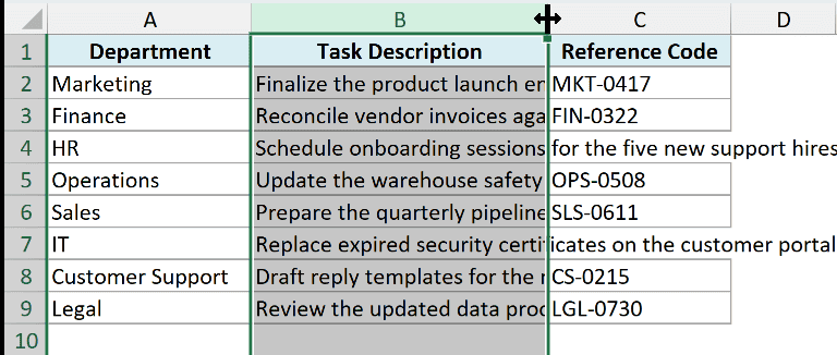
- Double-click the left mouse button or trackpad.
Excel changes the column width to fit the widest cell in column B.
The row method works the same way. Move the pointer to the bottom edge of the row header and double-click when the two-sided arrow appears.
AutoFit Multiple Columns, Rows, or the Entire Worksheet
You can also use the double-click method on several columns or rows at once. You need to select the complete columns or rows first.
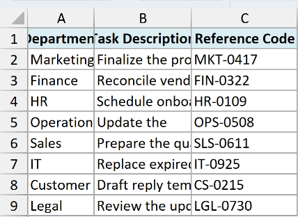
This time, both the Department and Task Description columns are too narrow for their contents.
Here are the steps to AutoFit both columns:
- Drag across the A and B column headers to select the entire columns.
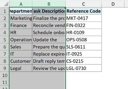
- Move the pointer to the right edge of either selected column header.
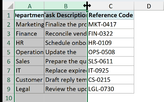
- Double-click when the pointer changes to a two-sided arrow.
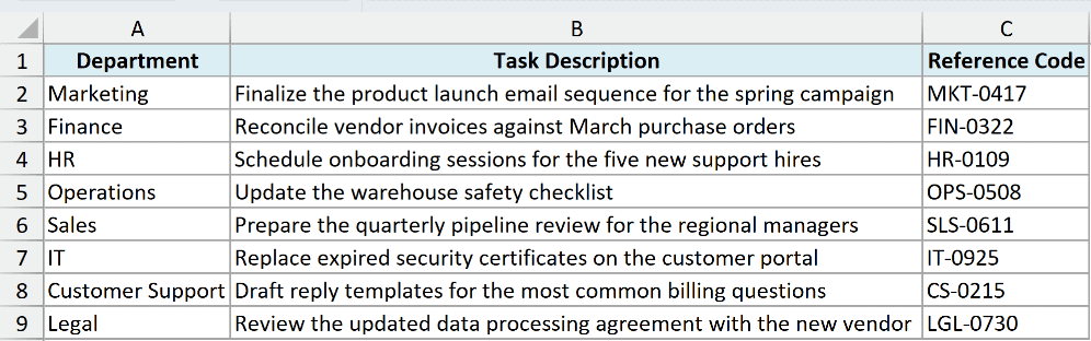
Excel AutoFits each selected column separately. Column A may end up narrower than column B because their contents have different widths.
The same selection rule applies to rows. Select the complete row headers before double-clicking a row boundary.
To AutoFit the entire task list worksheet, start by selecting every cell.
- Click the Select All button at the top-left corner of the worksheet, where the row numbers and column letters meet.
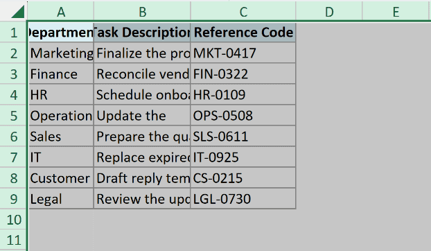
- Move the pointer to any column boundary and double-click to AutoFit all columns.
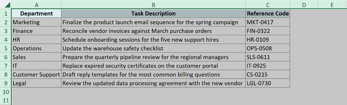
- Move the pointer to any row boundary and double-click to AutoFit all rows.
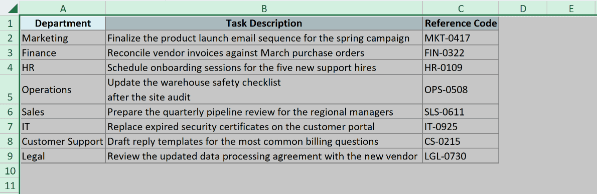
Pro Tip: Whole-sheet AutoFit gives each column and row a content-based size. It won’t make all cells uniform.
Follow along with the example file
AutoFit Excel Practice File.xlsx
Use the Excel Ribbon to Fit Text to Cells
The ribbon has separate commands for AutoFit Column Width and AutoFit Row Height.
Here, I want to AutoFit column B so every task description is visible.
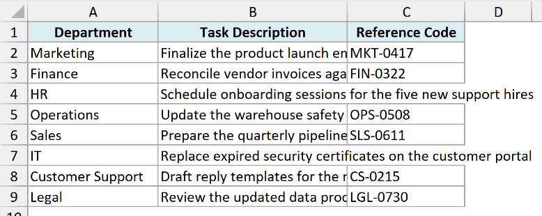
Here are the steps to AutoFit the column from the ribbon:
- Select column B.
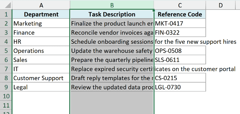
- Click the Home tab.
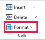
- In the Cells group, click Format, then click AutoFit Column Width.
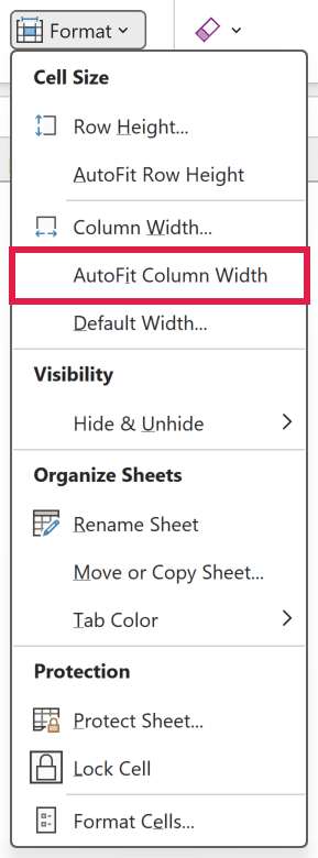
Excel immediately changes the selected column’s width.
Pro Tip: If you select only some cells instead of the whole column, AutoFit Column Width fits the column to those selected cells. This is handy when a long title in row 1 would otherwise make the column huge.
You can use the same ribbon menu to AutoFit the rows in the task list.
- Select the rows you want to AutoFit.
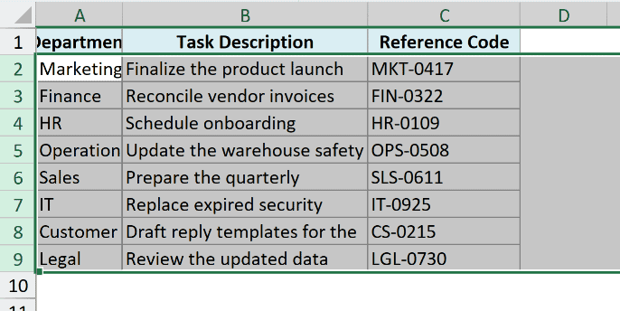
- On the Home tab, click Format in the Cells group, then click AutoFit Row Height.
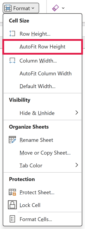
The mouse and ribbon methods work in current desktop versions of Excel. You can also use AutoFit in Excel for Mac and Excel for the web, although the ribbon may look slightly different.
AutoFit Shortcuts in Excel for Windows
If you prefer the keyboard, Excel for Windows has shortcuts for both AutoFit commands.
In this task list, the Department and Task Description columns need more room, while several wrapped descriptions need taller rows.
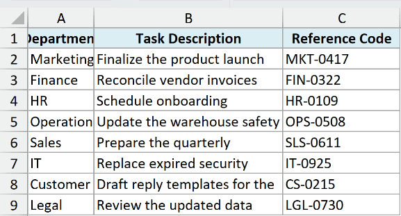
Below is the shortcut to AutoFit the selected column or columns:
Shortcut: Alt + H + O + I
Below is the shortcut to AutoFit the selected row or rows:
Shortcut: Alt + H + O + A
Select the complete row or column first. Then press the keys in succession, rather than holding all four keys down together.
These are Windows ribbon shortcuts. On a Mac or in Excel for the web, use the mouse or the AutoFit commands in the ribbon.
You can find more time-saving combinations in this list of keyboard shortcut options.
Can a Formula AutoFit Cells in Excel?
Here, a formula returns longer task descriptions in column B. As the results change, some text no longer fits inside the column.
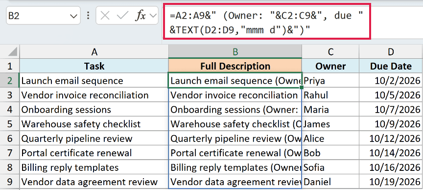
A worksheet formula can’t change a column’s width or a row’s height. It can return text or numbers, but it can’t change worksheet dimensions.
You can run one of the AutoFit methods above after a formula result changes. The VBA method below can resize columns after you type or paste data, but it won’t respond to formula-only recalculation.
AutoFit Columns Automatically as Data Changes Using VBA
VBA can AutoFit the affected columns whenever someone changes data on a worksheet.
I have a task list where new task descriptions are added regularly. I want Excel to resize each changed column without running AutoFit manually.
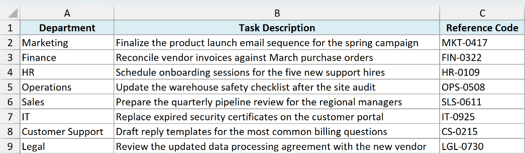
Here is the VBA code:
Private Sub Worksheet_Change(ByVal Target As Range)
    Target.EntireColumn.AutoFit
End SubHere are the steps to add it to the worksheet:
- Right-click the tab of the sheet you want to automate.
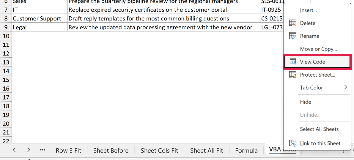
- Click View Code.
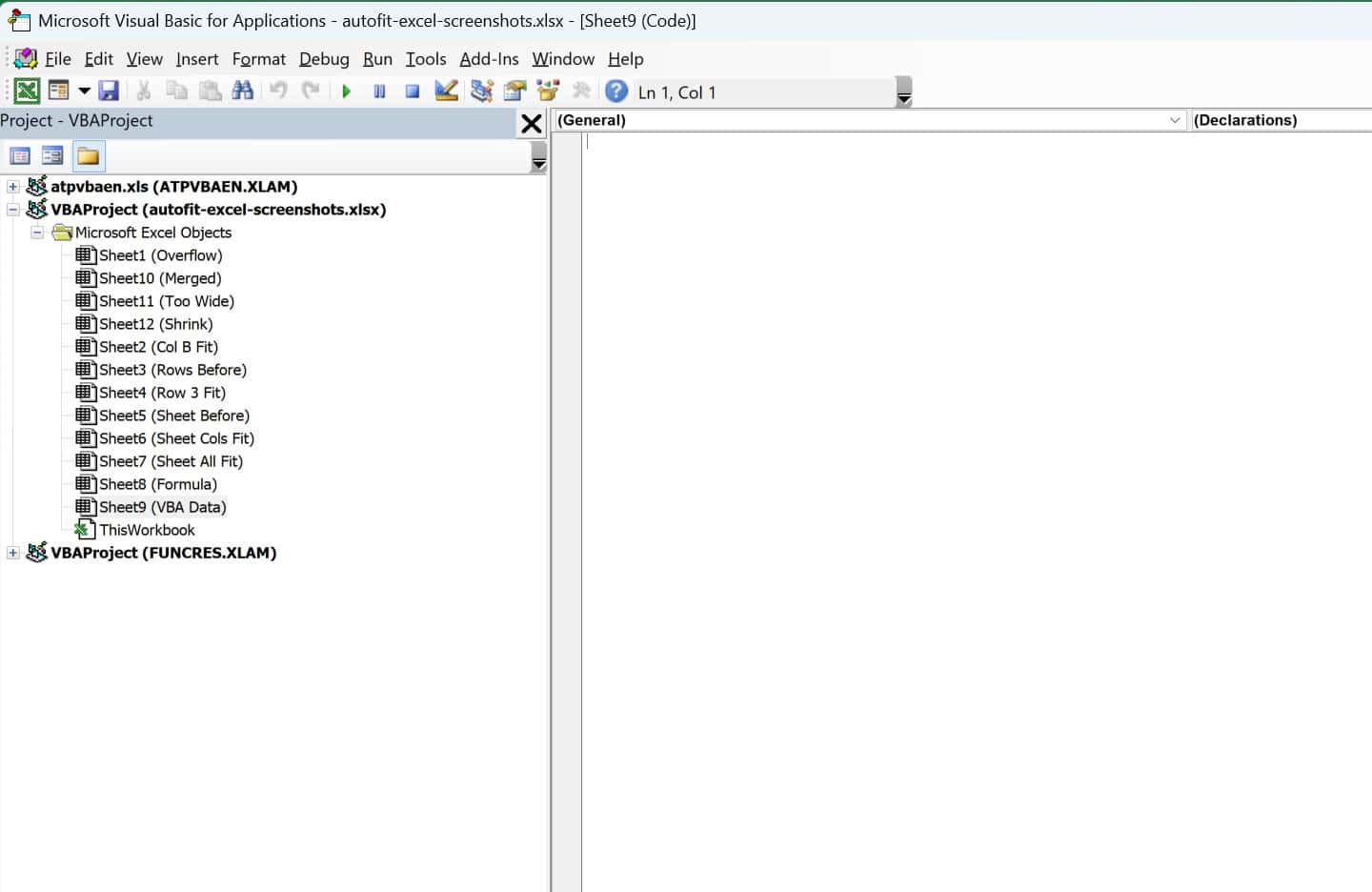
- Paste the code into the code window for that sheet.
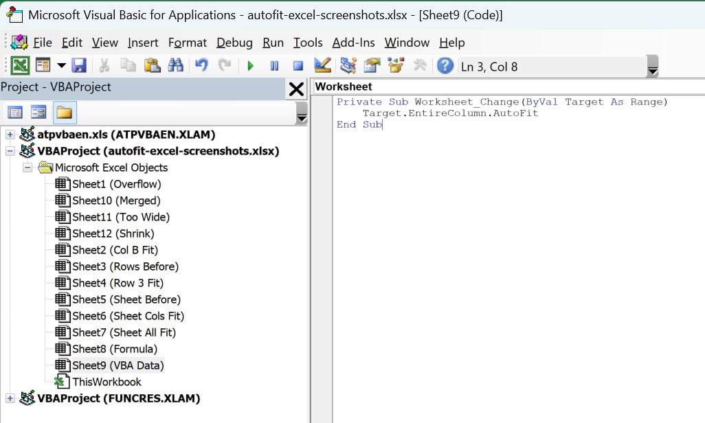
- Close the VBA Editor, return to Excel, and save the workbook as an Excel Macro-Enabled Workbook with the .xlsm extension.
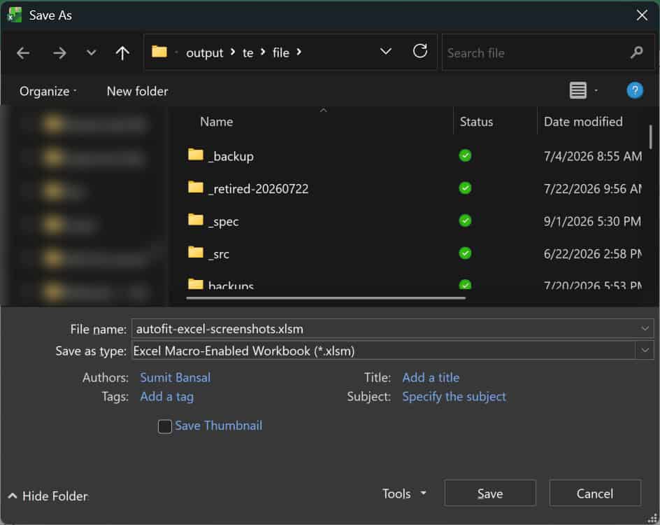
The code belongs in the sheet’s code module, not a standard module. It runs automatically, so you don’t need to press F5.
The Worksheet_Change event runs whenever you edit or paste a value on that sheet. Target represents the changed cells, and EntireColumn.AutoFit resizes their columns.
A formula result changing during recalculation doesn’t trigger this event. If you want the same behavior on another sheet, add the code to that sheet’s code module too.
Important: This event macro runs after every value edit on the sheet, which clears Excel’s undo history. In practice, Undo won’t work for edits on that sheet while the macro is active.
This method works in desktop Excel for Windows and Mac. Excel for the web can’t create, run, or edit VBA macros.
Follow along with the example file
AutoFit Excel Practice File.xlsx
Why AutoFit May Not Work in Excel
AutoFit usually works well with regular cells, but merged cells and wrapped text can affect the result.
The task list below has a merged heading and wrapped task descriptions. These settings can stop AutoFit or make the result look wrong.
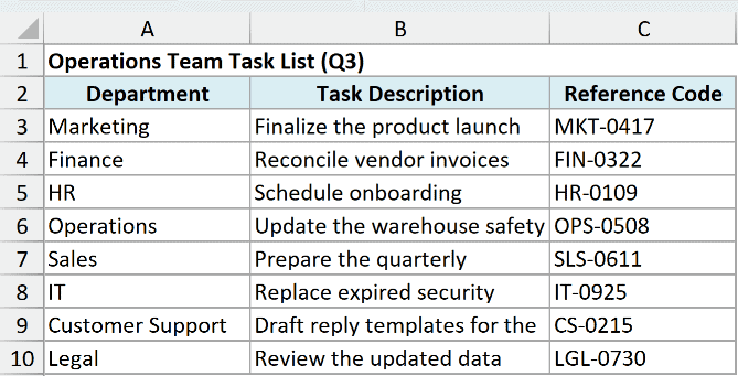
Merged cells
Excel can’t AutoFit a row or column that contains cells merged across other rows or columns. This limitation applies to current and older Excel versions.
Important: Unmerge the cells before using AutoFit, or right-click the column or row header and choose Column Width or Row Height.
Wrapped text
If you have applied text wrap, AutoFit Row Height normally expands the row to show every line.
A manually fixed row height or a merged cell can stop this adjustment. You may also see extra blank space above or below the wrapped text, even though the cell contains no extra spaces.
Changing the column width and running AutoFit Row Height again often removes this space. If it doesn’t, right-click the row header, choose Row Height, and type the value you want.
On a wrapped cell, AutoFit Column Width fits the column to the longest line as it’s currently wrapped, so the column can even get narrower. It won’t unwrap the text onto one line. Set the width first, then AutoFit the row height.
When AutoFit Makes a Column Too Wide
AutoFit uses the widest cell when calculating column width. One long task description can make the entire column much wider than you want.
In this example, one detailed task description causes column B to take up most of the worksheet.

Wrap Text keeps the content inside your chosen column width and displays it on multiple lines.
Set the width you want, turn on Wrap Text, and then use AutoFit Row Height. The separate Wrap Text guide covers the full method and its shortcuts.
If you want to hide the overflow instead of wrapping it, see Clip Text in Excel.
Use Shrink to Fit When the Column Width Must Stay Fixed
Shrink to Fit keeps the current column width and reduces a cell’s font size until its contents fit. It works best with short entries because longer text can become difficult to read.
Here, the Reference Code column has a fixed width, and one code is slightly too long.
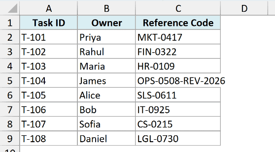
Here are the steps to apply Shrink to Fit:
- Select the cells containing the reference codes.
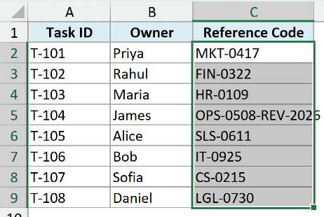
- Press Ctrl + 1 to open the Format Cells dialog box.
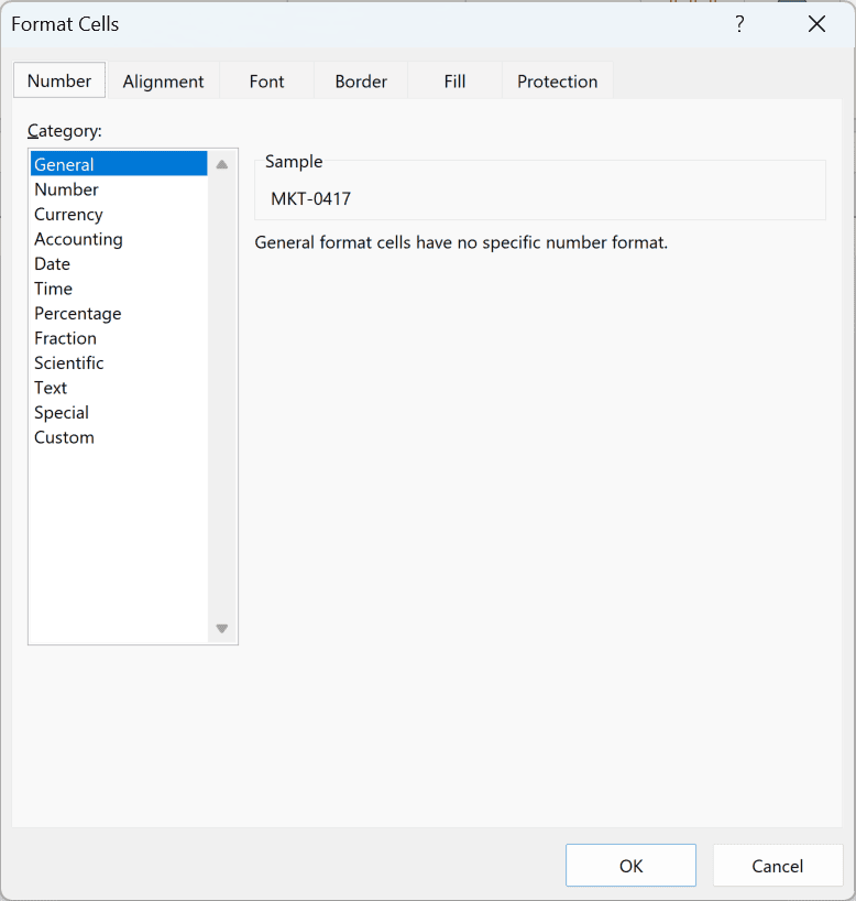
- Click the Alignment tab.
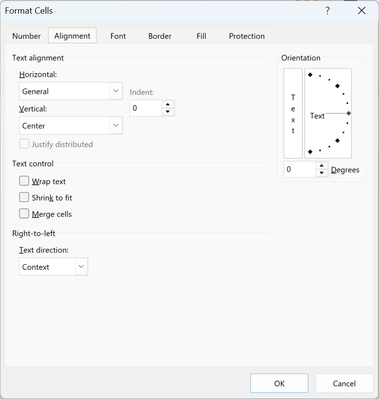
- Select Shrink to Fit under Text Control, then click OK.
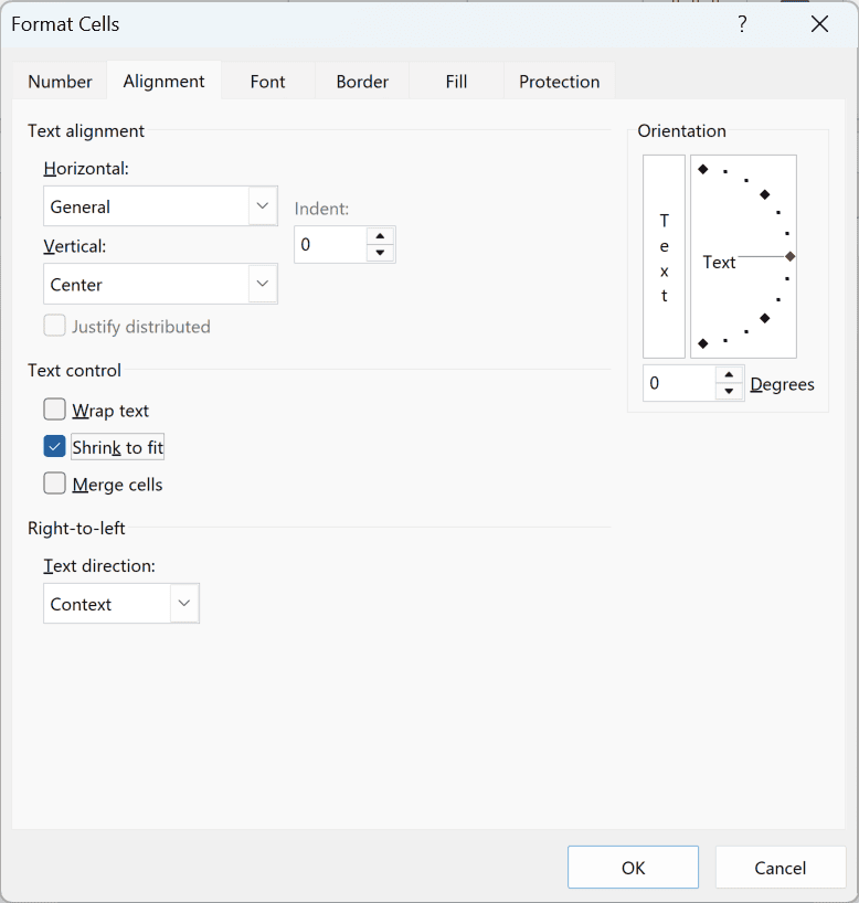
Excel reduces the font size so the selected content fits within the existing column width.
Important: Shrink to Fit can’t be used while Wrap Text is selected for the same cells.
Most of the time, I reach for the double-click method because it’s the quickest. If one long entry makes the column too wide, I’d use Wrap Text instead.
I hope you found this article helpful.
Other Excel Articles You May Also Like:
- How to Insert Line Break in Excel
- 7 Amazing Things Excel Text to Columns Can Do For You
- Add Bullet Points in Excel
- How to Lock Row Height & Column Width in Excel
- How to Change Row Height in Excel
- How to Copy Column Widths in Excel (Shortcut)
- How to Freeze Multiple Columns in Excel?
- How to Write Vertically in Excel
