

To hide formulas in Excel so that people only see the value, you need to turn on the Hidden option for those cells and then protect the worksheet.
When you share a normal Excel file with others, they are able to see and edit everything that the Excel file has.
If you don’t want them to change anything, you have the option to either protect the entire worksheet/workbook or protect certain cells that have important data (that you don’t want the user to mess up).
But even when you protect the worksheet, the end-user can still click on a cell and see the formula that’s used for calculations. If you want to hide the formula so that the users cannot see those, you can do that as well.
In this tutorial, I will show you how to hide formulas in Excel in a protected worksheet (so that it’s not visible to the user).
You’ll also see how to keep the rest of the sheet editable, how to bring the formulas back, and your options if you don’t want to protect the sheet.
One quick check first. If your cells are showing formulas instead of results, that’s usually the Show Formulas view, which you can turn off by pressing Control + ` (the grave accent key, usually above the Tab key).
If that doesn’t fix it, have a look at Excel Showing Formula Instead of Result.
So let’s get started!
Follow along with the example file
Hide Formulas in Excel.xlsx
How to Hide All Formulas in Excel
When you have a formula in a cell, a user can see the formula in two ways:
- By double-clicking on the cells and getting into the edit mode
- By selecting the cell and seeing the formula in the formula bar
When you hide the formulas and protect the sheet (as we’ll soon see how), the users won’t be able to edit the cell as well as not be able to see the formula in the formula bar.
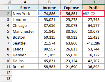
Suppose you have a data set as shown below (the Hide All Formulas sheet in the example file) where you have the formula in column D, and you want to hide these formulas so that only the profit values show.
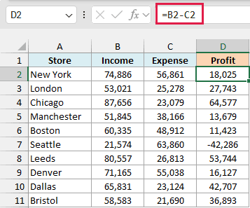
Below are the steps to hide all the formulas in column D:
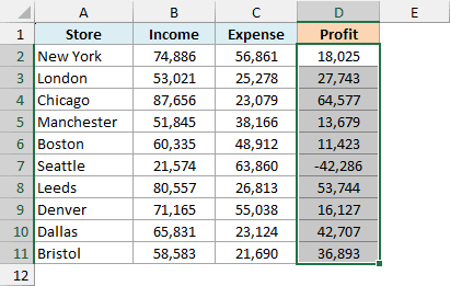
- Select the cells in column D that have the formula that you want to hide
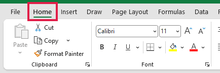
- Click the ‘Home’ tab
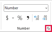
- In the ‘Number’ group, click on the dialog box launcher (it’s the small tilted arrow icon at the bottom right of the group)
Pro Tip: You can skip steps 2 and 3 by holding the Control key and pressing the 1 key (or the Command key and the 1 key if using Mac). This opens the same Format Cells dialog box.
- In the ‘Format Cells’ dialog box that opens up, click the ‘Protection’ tab
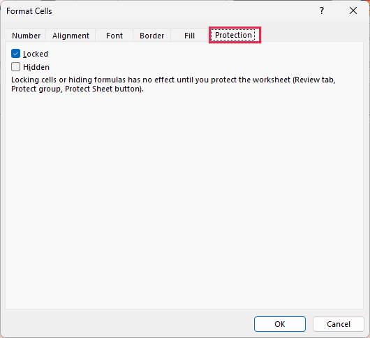
- Check the Hidden option
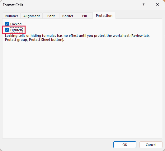
- Click OK
At this point, nothing is hidden yet. The Protection tab says so itself: “Locking cells or hiding formulas has no effect until you protect the worksheet.”
So that’s what we’ll do next.
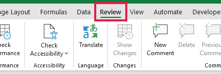
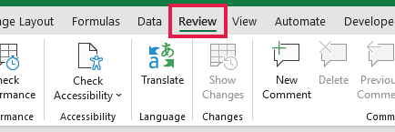
- Click the Review tab in the ribbon
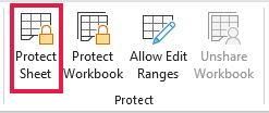
- In the Protect group, click on the Protect Sheet option
- In the Protect Sheet dialog box, enter the password that would be needed if you want to unlock the worksheet (in case you don’t want to apply a password, you can leave this blank)
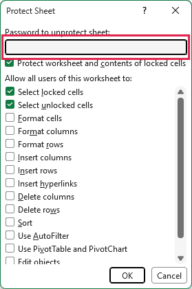
- Click OK (if you entered a password, Excel asks you to type it again, so re-enter it and click OK)
The above steps would protect the entire worksheet in such a way that if you click on a cell that has a value you would see the value in the formula bar.
But if you click on a cell that has a formula, no formula would be shown in the formula bar.
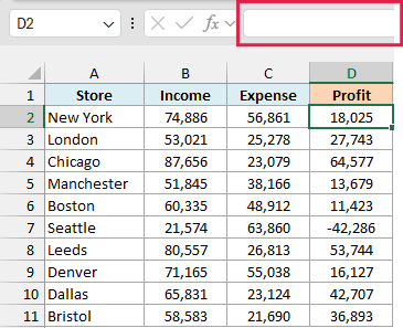
And since the worksheet is protected, you would not be able to double-click on the cell and get into the edit mode (so the formula is hidden that way as well). Excel shows a message saying that the cell is on a protected sheet.
The whole sheet gets locked here because every cell in Excel has the Locked property turned on by default, and protecting the sheet enforces that setting. So you can’t edit the Income and Expense values either until you unprotect the sheet.
People sometimes try two other ways of getting to a formula, and they don’t work on these cells either. If someone turns on Show Formulas, the hidden cells look blank, and if they copy a cell and paste it somewhere else, they only get the value.
Hiding formulas this way works in Excel for Microsoft 365, Excel 2024, 2021, 2019, and 2016.
While this method works fine, you need to know that the sheets/cells that are protected in Excel can easily be unlocked by the user. Without a password, anyone can turn the protection off from the Review tab.
Any tech-savvy user can easily break into your protected workbooks (a simple Google search will give them multiple ways to break the protected worksheet). It’s not straight-forward, but it’s not too hard.
But if you’re working with less tech-savvy users, adding a password should be enough.
A password still isn’t real security, though. Your formula stays in the saved file as plain text, and Microsoft itself says that worksheet protection isn’t a security feature.
So if a formula truly must stay private, share a copy that has only the values (more on this later in this tutorial).
Also read: How to Lock Formulas in Excel
How to Only Hide Formulas in Excel (And Keep Rest of the Cells Editable)
In the above method, I showed you how to protect the entire worksheet (including the cells that don’t have a formula in them).
But what if you don’t want to protect the entire worksheet? What if you only want to protect the cells that have formulas and hide these formulas from the user.
This could be the case when you want the users to input data (such as in a data entry form) but not be able to edit the formula or see it. This can easily be done as well.
Unlike the previous method, where we protected all the cells in the worksheet, in this method only the cells that have the formulas stay locked (the sheet still gets protected, but the other cells are unlocked first). The rest of the worksheet would remain open for the user to edit.
Follow along with the example file
Hide Formulas in Excel.xlsx
Suppose you have a data set as shown below (the Keep Inputs Editable sheet in the example file) where you only want to lock and hide the formulas in column D, and keep the other cells editable.
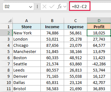
For a cell to be protected, it needs to have the ‘Locked’ property enabled, as well as the protection enabled from the ribbon. Only when both of these happen does a cell truly become locked (i.e., can’t be edited).
This also means that if you disable the lock property for a few cells, these could still be edited after you protect the worksheet.
We will use this concept where we will disable the locked property for all the cells except the ones that have formulas in them. Let’s see how to do this.
Step 1: Disable the Lock Property for All the Cells
So, we first need to disable the Locked property for all the cells, including the ones with formulas (so that these stay editable after we protect the sheet). In Step 2, we’ll turn it back on for only the cells that have formulas.
Below are the steps to do this:
- Select all the cells in the worksheet (you can do this by clicking on the gray triangle at the top left part of the sheet)
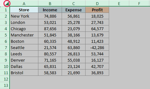
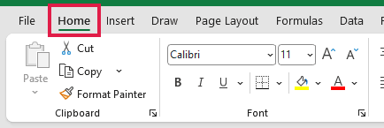
- Click the Home tab
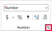
- In the Number group, click on the dialog box launcher
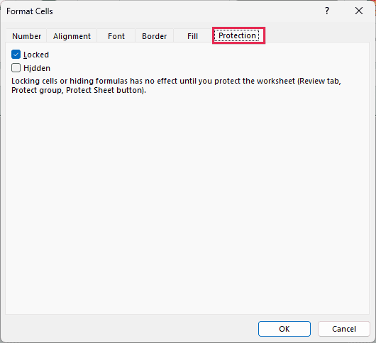
- In the Format Cells dialog box, click on the ‘Protection’ tab
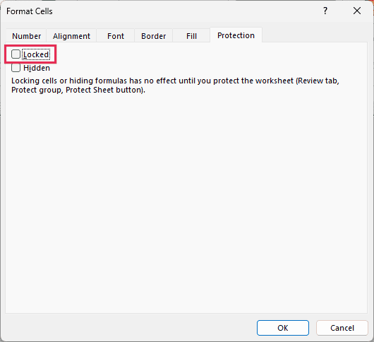
- Uncheck the Locked option
- Click OK
The above steps have disabled the locked property for all the cells in the worksheet.
Now, even if I go and protect the sheet using the option in the ribbon (Review >> Protect Sheet), the cells would not be locked and you can still edit the cells.
Step 2: Enable the Locked and Hidden Property Only for Cells with Formulas
To hide the formula from all the cells in the worksheet, I now need to somehow identify the cells that have the formula and then lock these cells.
And while locking these cells, I would make sure that the formula is hidden from the formula bar as well.
Below are the steps to hide formulas:
- Select all the cells in the worksheet (you can do this by clicking on the gray triangle at the top left part of the sheet)
- Click the Home tab
- In the Editing group, click on the Find & Select option
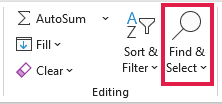
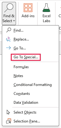
- Click on the ‘Go To Special’ option
- In the Go To Special dialog box, click on the Formulas option
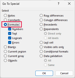
- Click OK. This will select all the cells that have a formula in them
Go To Special doesn’t work on a protected sheet, so this has to happen before you protect the worksheet in Step 3.
- With the cells with formulas selected, hold the Control key and then press the 1 key (or the Command key and the 1 key if using Mac). This will open the Format Cells dialog box
- Click on the ‘Protection’ tab
- Make sure ‘Locked’ and ‘Hidden’ options are checked
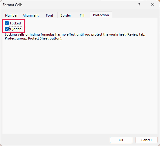
- Click OK
You need both options because they do different jobs. Locked stops people from changing the formula, and Hidden stops them from seeing it, so a cell with only Hidden checked keeps its formula out of view but can still be overwritten.
Also read: Highlight Cells With Formulas in Excel
Step 3: Protecting the Worksheet
In the process so far, the Locked property is disabled for all the cells except the ones that have a formula in them.
So now, if I protect the entire worksheet, only those cells would be protected that have a formula (as you need the Locked property to be enabled to truly lock a cell).
Here are the steps to do this:
- Click the Review tab
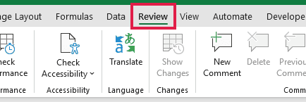
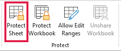
- In the Protect group, click on the ‘Protect Sheet’ option
- In the Protect Sheet dialog box, enter the password (optional)
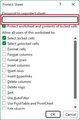
Pro Tip: In the same dialog box, you can also uncheck ‘Select locked cells’. Then nobody can even click on the formula cells, and they can only select the cells you left unlocked.
- Click OK (if you entered a password, re-enter it when Excel asks and click OK)
The above steps would lock only those cells that have a formula in them and at the same time hide the formula from the users.
The users won’t be able to double-click and get into the edit mode as well as see the formula in the formula bar. They can still change the Income and Expense values, and the Profit values update as usual.
Also read: Excel Formulas Not Working
How to Hide a Spilled Formula in Excel
The method above needs one small change when your results come from a single spilling formula. That’s one formula in the top cell that fills the whole column on its own (available in Excel 365, 2024, and 2021).
Below is the same data set (the Spilled Formula sheet in the example file), where one formula in cell D2 fills column D, and I want to hide it while keeping the rest of the sheet editable.
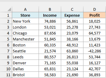
Here is the formula in cell D2:
=B2:B11-C2:C11
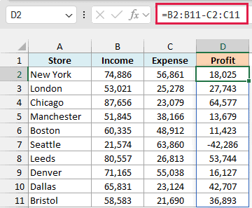
The catch is in Step 2 above. Go To Special only selects the first cell of a spill, so here it selects D2 and leaves D3:D11 out.
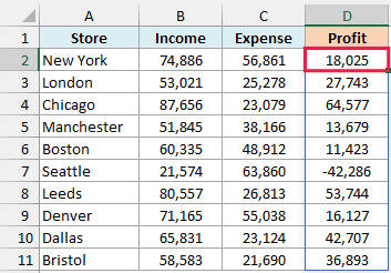
If you follow the method as written and protect the sheet, the formula stays hidden in all of these cells, because D3:D11 don’t have a formula of their own (they only show what D2 returns).
But D3:D11 stay unlocked, because Step 1 turned off their Locked property and Step 2 never turned it back on.
Important: If you lock only D2, someone can still type in a cell such as D3 on the protected sheet. A spilling formula needs all the cells it fills to be empty, so D2 then shows a #SPILL! error and the other results in the column disappear.
To avoid this, lock the whole spill range yourself. Below are the steps to do this:
- Follow Step 1 above to disable the Locked property for all the cells
- Select all the cells in the spill range (D2:D11 in this example)
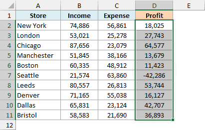
- Hold the Control key and press the 1 key (or the Command key and the 1 key if using Mac)
- Click on the ‘Protection’ tab
- Make sure ‘Locked’ and ‘Hidden’ options are checked
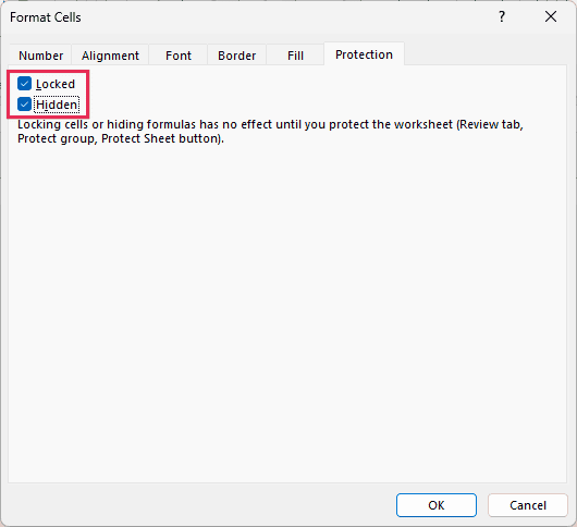
- Click OK
- Follow Step 3 above to protect the worksheet
Now every cell in the spill range is locked, so nobody can type over the results. The Income and Expense values stay editable, and the formula still recalculates when they change.
How to Unhide Formulas in Excel
If you’ve hidden formulas and now need them back, you only need to unprotect the sheet. Here are the steps:
- Click the Review tab
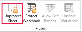
- In the Protect group, click on the Unprotect Sheet option (and enter the password if the sheet has one)
The formulas now show up in the formula bar again. But the Hidden option is still checked for those cells, so the formulas would get hidden again the next time you protect the sheet.
If you want to protect the sheet later and keep these formulas visible, you also need to clear the Hidden option. Here are the steps:
- Select the cells that have the formulas
- Hold the Control key and press the 1 key (or the Command key and the 1 key if using Mac)
- Click on the ‘Protection’ tab
- Uncheck the Hidden option
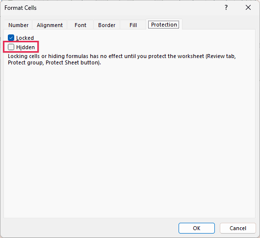
- Click OK
How to Hide Formulas Without Protecting the Worksheet
If you’re wondering whether you can hide the formulas in Excel without protecting the sheet, unfortunately, you can’t.
While you can get this done by using a complex VBA code, it would be unreliable and can lead to other issues. Here is an article that shares such a code (use it if you really really can’t do without it).
This kind of code swaps the formula for its value when you select the cell. It can’t run with macros turned off, so anyone who opens the file that way can click on the cell and see the formula.
As of now, the only built-in way to hide the formulas in Excel is to protect the sheet and also make sure that the Hidden property is enabled for the cells that have the formula.
There are a few workarounds that can get you close, as long as you know where each one falls short.
If people only need the results, you can remove the formulas and keep the data in a copy of the file. This is the only option here where the formula really isn’t there for anyone to find, but the copy no longer recalculates.
You can also keep the real formula on a separate sheet (say, a sheet named Calc). The visible cell still shows the result, but its formula bar only shows a reference like =Calc!D2.
Then make that sheet very hidden, which is different from the regular Hide because it can’t be unhidden from the regular menu. Someone comfortable with the VB Editor can still bring it back.
Another option is to hide the formula bar, but this setting applies to your own Excel rather than to the file. Anyone else opening the file still sees their own formula bar, and even on your computer, double-clicking the cell shows the formula.
One option that doesn’t help here is the custom number format ;;;. It hides the result in the cell, but the formula still shows up in the formula bar, which is the opposite of what we want.
So these are the ways you can hide formulas in Excel so that people only see the values.
I hope you found this tutorial useful.
Other Excel Articles You May Also Like:

thank you very much it is helpful for me
Thank you! This worked and was helpful.