

If you’ve tried giving a range to a function such as EOMONTH or the WORKDAY function, expecting it to spill the results, you’ve probably run into the #VALUE! error instead.
And this is because some older Excel functions were never taught how to handle a range of cells as an input. But nothing to worry about.
There is a simple trick that forces these functions to spill, and in this article I’ll show you how it works and why.
I also covered this trick in the video below, so you can watch that as well.
Why Some Excel Functions Refuse to Spill
Most functions in Excel 365 are happy to take a range and spill the results.
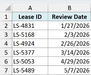
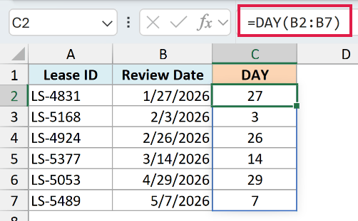
For example, below I have a dataset with lease IDs in column A and their review dates in column B, and I want the day number for each date.
I can give the DAY function the entire range, and it spills the result for every date in one go:
=DAY(B2:B7)
Now watch what happens when I try the exact same thing with the EOMONTH function, which should give me the last day of the month for each date:
=EOMONTH(B2:B7,0)
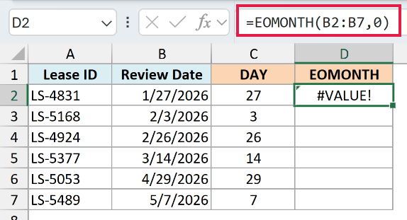
Instead of spilling, it gives me the #VALUE! error. The formula is fine, the dates are fine, and yet EOMONTH refuses to work with the range.
Here is a little bit of Excel history to explain this. EOMONTH and a bunch of other functions were originally part of the Analysis ToolPak, an add-in that shipped with older versions of Excel. Microsoft later made them native Excel functions.
When dynamic arrays arrived in Excel 365, these functions kept their old programming. They still expect a single cell as the input, so when you hand them a range, they throw the #VALUE! error instead of spilling.
Here is the whole story at a glance:
The Fix: Add a Plus Sign Before the Range
Here is the trick. Take the same EOMONTH formula that failed, and add a plus sign right before the range:
=EOMONTH(+B2:B7,0)
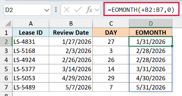
That one character fixes it. The formula now spills and gives me the end-of-month date for every review date in the dataset.
How does this trick work?
The plus sign is a math operator, so Excel has to evaluate +B2:B7 before it can pass anything to EOMONTH. That evaluation converts the range reference into an array of values.
And while these older functions cannot handle a range reference, they can handle an array. Once they get an array, Excel’s dynamic array engine takes over, runs the function on each value, and spills the results.
You Can Also Add +0 After the Range
If the plus sign in front feels odd to you, adding a zero after the range does the same job:
=EOMONTH(B2:B7+0,0)
Both versions work exactly the same way, so use whichever one you find easier to remember.
I prefer the plus sign in front since it is one less character and I don’t confuse it with the other arguments.
Since these results are dates, you may see serial numbers such as 46081 instead of dates in the spilled range.
Just select the range and change the format to a date format (Home tab, Number Format drop-down).
Excel Functions That Won’t Spill (the Full List)
EOMONTH is not the only function with this problem. Others such as EDATE, NETWORKDAYS, and RANDBETWEEN behave the same way.
I tested the common ones in Excel 365, and all of the functions below give the #VALUE! error with a range but spill fine with the plus sign trick.
| Function | Fails | Works |
|---|---|---|
| EOMONTH | =EOMONTH(B2:B7,0) | =EOMONTH(+B2:B7,0) |
| EDATE | =EDATE(B2:B7,1) | =EDATE(+B2:B7,1) |
| WORKDAY | =WORKDAY(B2:B7,10) | =WORKDAY(+B2:B7,10) |
| WORKDAY.INTL | =WORKDAY.INTL(B2:B7,10) | =WORKDAY.INTL(+B2:B7,10) |
| NETWORKDAYS | =NETWORKDAYS(B2:B7,TODAY()) | =NETWORKDAYS(+B2:B7,TODAY()) |
| NETWORKDAYS.INTL | =NETWORKDAYS.INTL(B2:B7,TODAY()) | =NETWORKDAYS.INTL(+B2:B7,TODAY()) |
| YEARFRAC | =YEARFRAC(B2:B7,TODAY()) | =YEARFRAC(+B2:B7,TODAY()) |
| WEEKNUM | =WEEKNUM(B2:B7) | =WEEKNUM(+B2:B7) |
| ISEVEN | =ISEVEN(B2:B7) | =ISEVEN(+B2:B7) |
| ISODD | =ISODD(B2:B7) | =ISODD(+B2:B7) |
| MROUND | =MROUND(B2:B7,5) | =MROUND(+B2:B7,5) |
| QUOTIENT | =QUOTIENT(B2:B7,2) | =QUOTIENT(+B2:B7,2) |
| RANDBETWEEN | =RANDBETWEEN(B2:B7,100) | =RANDBETWEEN(+B2:B7,100) |
| CONVERT | =CONVERT(B2:B7,"m","ft") | =CONVERT(+B2:B7,"m","ft") |
A quick note here. Some lists on the internet also include functions such as PMT or ISOWEEKNUM. When I tested these in the current version of Excel 365, they spill just fine with a plain range, so you don’t need the trick for them.
Using MAP as an Alternative
The plus sign trick works, but =EOMONTH(+B2:B7,0) does look a little cryptic. If a colleague opens your file, they may wonder what that lonely plus sign is doing there.
If you’d rather use a pattern that makes the intent obvious, and one that works with any function, you can use the MAP function.
It runs a function on each cell of a range and spills the results. Note that MAP is only available in Excel 365, not in Excel 2021.
Here is the MAP version of our EOMONTH formula:
=MAP(B2:B7,LAMBDA(d,EOMONTH(d,0)))
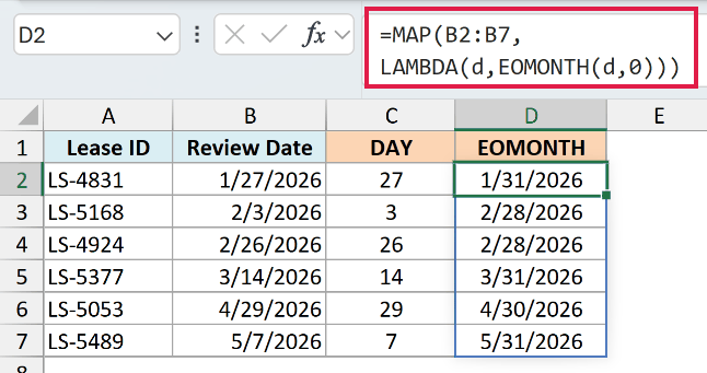
How does this formula work?
MAP takes each value in B2:B7, hands it to the LAMBDA one at a time as d, and EOMONTH only ever sees a single value. Since that is exactly what EOMONTH was built for, there is nothing left to trip it up.
This is a bit more typing than the plus sign, so I use MAP only when the simple trick doesn’t apply.
What About Excel Tables?
If your data is in an Excel Table, you don’t have to worry about any of this. Formulas can’t spill inside an Excel Table anyway, so the question never comes up.
Below I have the same lease data, but this time formatted as an Excel Table.
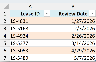
When I add a column and refer to a single date cell, Excel uses a structured reference such as [@[Review Date]] and automatically fills the formula down the whole column:
=EOMONTH([@[Review Date]],0)
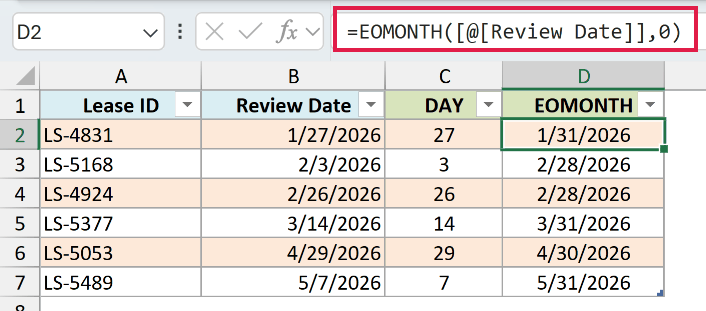
So inside a Table, EOMONTH and its stubborn friends behave perfectly. The plus sign trick is only needed when you work with these functions in a normal range and want the result as a spilled dynamic array.
Things to Keep in Mind
- This trick needs a version of Excel that supports dynamic arrays, which means Excel 365 or Excel 2021 and later. In older versions there is no spilling at all.
- The plus sign isn’t the only operator that works. Multiplying the range by 1, as in
=EOMONTH(B2:B7*1,0), or using a double negative, as in=EOMONTH(--B2:B7,0), does the same conversion. I stick with the plus sign since it’s the shortest. - If the spilled result shows serial numbers instead of dates, apply a date format to the spill range. The trick returns date serial numbers, and Excel does not always format them as dates automatically.
- You can nest the trick inside other functions. For example,
=TEXT(EOMONTH(+B2:B7,1),"mmm yyyy")spills the month names for the next month. - If you get a #SPILL! error after applying the trick, some cells below the formula already have data in them. Clear those cells and the formula will spill.
In this article, I showed you why functions such as EOMONTH and WORKDAY give the #VALUE! error with a range, and how a simple plus sign forces them to spill. I hope you found this article helpful.
Other Excel Articles You May Also Like:
