

The PERCENTRANK.EXC function tells you where a number stands within a list, as a percentile rank between 0 and 1. A result of 0.7 (70%) means the number sits about 70% of the way up the list.
The EXC in the name stands for exclusive. It means the smallest value never gets 0% and the largest never gets 100%, which can look a bit odd the first time you see it.
In this tutorial, I will show you why that happens, how to rank a number that isn’t in your list, and what to do when the formula returns #N/A.
Follow along with the example file
PERCENTRANK.EXC Function Examples.xlsx
PERCENTRANK.EXC Function Syntax
Here is the syntax of the PERCENTRANK.EXC function:
=PERCENTRANK.EXC(array, x, [significance])
- array – The list of numbers you want to compare against. It doesn’t need to be sorted, and any text or blank cells in it are ignored.
- x – The value you want to rank. It doesn’t have to be in the array, but it has to fall between the smallest and largest values in it.
- significance – (Optional) The number of digits to keep in the result. If you leave it out, Excel keeps three digits (such as 0.538).
The x argument can also be a range of values. In Excel 365 and Excel 2021 or later, you then get one rank for each value, and the results spill into the cells below.
The significance argument cuts off the extra digits instead of rounding them. It has to be 1 or more, otherwise the formula returns a #NUM! error.
The PERCENTRANK.EXC function works in Excel 2010 and later, including Microsoft 365, Excel 2024, 2021, 2019, 2016, Excel for Mac, and Excel for the web.
When to Use the PERCENTRANK.EXC Function
Use this function when you need to:
- See where a score, price, or bill stands compared with the rest of a list
- Get percentile ranks where no value is pinned at exactly 0% or 100%
- Check where a new value would fall among the values you already have
- Rank a value against only one group within a larger list
Let me show you a few practical examples of how to use PERCENTRANK.EXC in Excel.
Example 1: Find the Percentile Rank of Every Value in a List
Let’s start with a simple example.
Below is a list of nine bowlers with their scores from one league night, and I want to show each bowler’s percentile rank in column C.
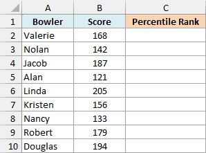
Here is the formula:
=PERCENTRANK.EXC(B2:B10,B2:B10)
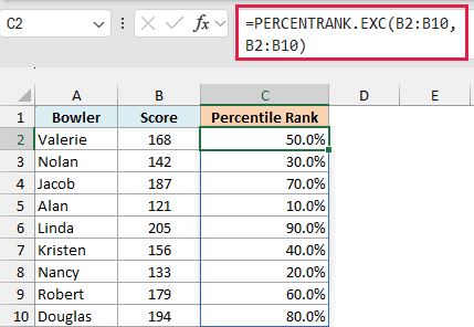
The first B2:B10 is the list of scores to compare against, and the second B2:B10 is the scores we want to rank. Since the second argument is a whole range, you get one result per bowler, and the results spill down column C.
Linda has the highest score (205), but she gets 90%, not 100%. Alan has the lowest score (121), and he gets 10%, not 0%.
That’s the exclusive part. PERCENTRANK.EXC counts how many values are below the one you’re ranking, adds 1, and then divides by the number of values plus 1.
For Valerie’s 168, four scores are lower, so her rank is (4 + 1) divided by (9 + 1), which is 0.5, or 50%. With nine scores, the ranks go up in steps of 10%, from 10% for the lowest to 90% for the highest.
Important: Make sure the cells below C2 are empty before you enter the formula. If anything blocks the range where the results need to go, Excel returns a #SPILL! error instead.
If you are using Excel 2019 or earlier, enter the below formula in cell C2 and then copy it down the range:
=PERCENTRANK.EXC($B$2:$B$10,B2)
The dollar signs make B2:B10 an absolute reference, so the list of scores stays fixed as you copy the formula down, while B2 changes to B3, B4, and so on. The same approach works for the other spilling formulas in this article.
Example 2: Percentile Rank of a Value That’s Not in the List
Here’s another practical scenario.
Below are the nightly rates of nine hotels in a city, and I want to see how a quoted rate of $185 (in cell D2) ranks against them in cell E2.
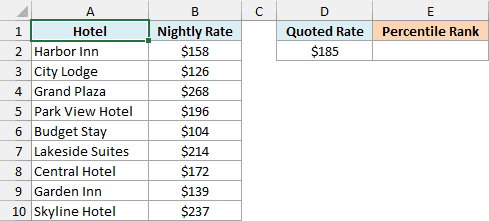
Here is the formula:
=PERCENTRANK.EXC(B2:B10,D2)
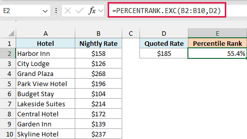
The result is 55.4%, even though $185 isn’t one of the nine rates. It falls between Central Hotel’s $172, which ranks at 50%, and Park View Hotel’s $196, which ranks at 60%.
So Excel fills in the gap proportionally (this is called interpolation). $185 is about 54% of the way from $172 to $196, so its rank lands about 54% of the way from 50% to 60%, which gives 55.4%.
This is handy when you want to check a new number without adding it to your list. Adding it would change the list itself, and with it the rank of every other hotel.
Example 3: Control the Decimals With the significance Argument
Sometimes you want fewer digits in the result.
Below are the electricity bills for each month of a year, and I want each bill’s percentile rank in column C, and a two-digit version of the same rank in column D.
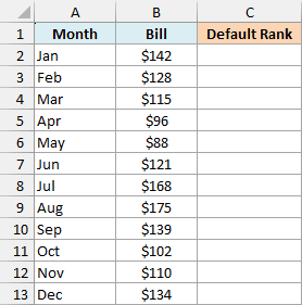
Here is the formula for column C:
=PERCENTRANK.EXC(B2:B13,B2:B13)
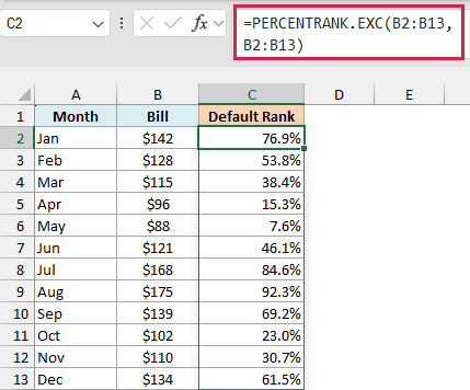
With 12 bills, every rank is a fraction of 13, so most of them don’t come out even. Excel keeps three digits by default, so August’s $175 bill (the highest) gets 0.923, shown as 92.3%.
Now here is the formula for column D:
=PERCENTRANK.EXC(B2:B13,B2:B13,2)
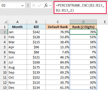
The 2 at the end is the significance argument, and it tells Excel to keep only two digits. January’s rank of 0.769 becomes 0.76, which shows as 76%.
Notice that it’s 76%, not 77%. The significance argument cuts off the extra digits instead of rounding, which is why February also drops from 53.8% to 53%.
Pro Tip: If you only want shorter numbers on screen, leave significance out and change the cell’s number format instead. Formatting rounds what you see (0.769 shows as 77%) and keeps every digit for later calculations.
Example 4: How PERCENTRANK.EXC Handles Tied Values
Now let’s look at what happens when the same value shows up more than once.
Below are the push-up counts of ten people from a fitness test, and I want each person’s percentile rank in column C.
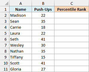
Here is the formula:
=PERCENTRANK.EXC(B2:B11,B2:B11)
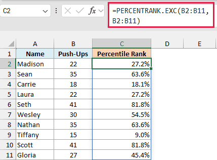
Tied values always get the same rank. Madison and Laura both did 22 push-ups, so both get 27.2%.
Excel uses the lower position for a tie. Two people did fewer than 22 push-ups, so the rank for 22 is (2 + 1) divided by (10 + 1), which is 0.272 after Excel drops the extra digits.
This matters most at the top of the list. Seth and Scott tied for the highest count (41), and both get 81.8%, so nobody in this list gets 90.9%, the rank a single top score would get among ten values.
So don’t assume the highest value always gets the highest possible rank. When the top value is repeated, every copy gets the rank of the lowest position in the tie, no matter which row it’s in.
Example 5: Why PERCENTRANK.EXC Returns #N/A (and How to Handle It)
Now let’s look at a case where the formula returns an error.
Below is a list of used bikes for sale with their prices, and I want to rank three new listings from column D against them in column E.
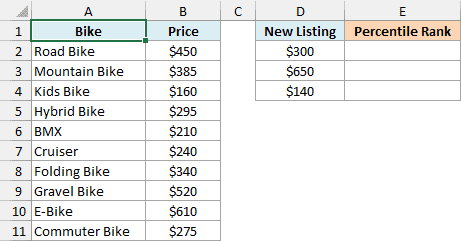
Here is the formula:
=PERCENTRANK.EXC(B2:B11,D2:D4)
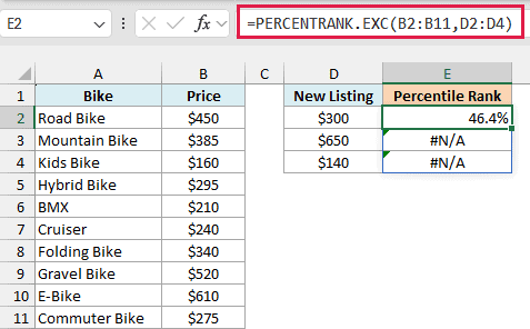
The $300 listing gets 46.4%, but the other two return #N/A. The $650 listing costs more than the most expensive bike in the list ($610), and the $140 listing costs less than the cheapest one ($160).
PERCENTRANK.EXC can only rank a value that falls between the smallest and largest values in the list. Outside that range, there’s nothing to interpolate between, so the function returns #N/A.
A value equal to the lowest or highest price is fine, because it’s in the list. A $160 listing, for example, would get the lowest rank instead of an error.
If you’d rather show a message than an error, wrap the formula in the IFNA function. Enter this formula in cell F2:
=IFNA(PERCENTRANK.EXC(B2:B11,D2:D4),"Outside range")
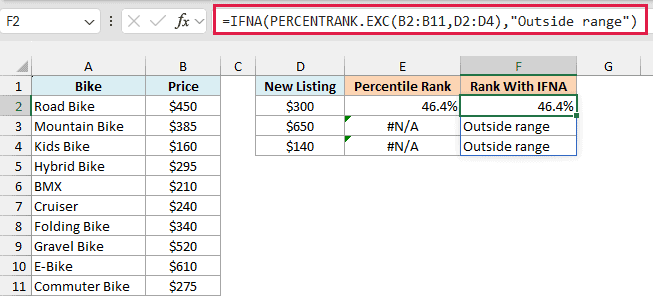
IFNA catches only the #N/A errors and shows “Outside range” instead, while the $300 listing keeps its 46.4% rank.
I used IFNA rather than the IFERROR function on purpose. IFERROR catches every type of error, including the #VALUE! error you get if someone types text such as “N/A” into column D.
With IFERROR, that typing mistake would hide behind “Outside range”. IFNA lets the #VALUE! error show, so you know there’s something to fix.
Example 6: Find the Percentile Rank Within One Group (With FILTER)
Let’s step it up with a more advanced use case.
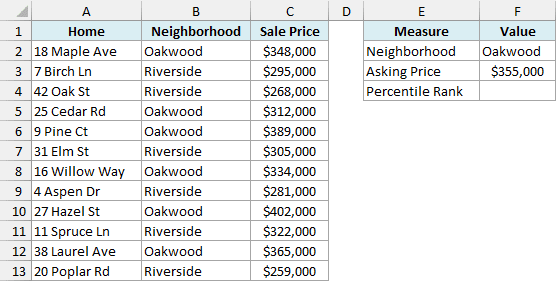
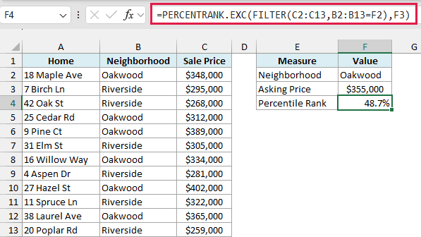
Below is a list of recent home sales from two neighborhoods, and I want to see how an asking price of $355,000 (in cell F3) ranks against only the homes in the neighborhood in cell F2 (Oakwood), with the result in cell F4.
Here is the formula:
=PERCENTRANK.EXC(FILTER(C2:C13,B2:B13=F2),F3)
How this formula works:
- FILTER(C2:C13,B2:B13=F2) returns only the sale prices of the homes in the neighborhood named in F2, which gives us the six Oakwood prices.
- PERCENTRANK.EXC then ranks the asking price in F3 against those six prices instead of all twelve.
The result is 48.7%, so $355,000 sits just below the middle of what Oakwood homes sold for. Every Riverside home sold for less than $355,000, so ranking against the full list would push the same price much higher than where it really stands in Oakwood.
The FILTER function needs Excel 365 or Excel 2021 and later. If you are using Excel 2019 or earlier, enter the below formula in cell F4 and press Control + Shift + Enter:
=PERCENTRANK.EXC(IF(B2:B13=F2,C2:C13),F3)
The IF part keeps the Oakwood prices and turns every other price into FALSE, which PERCENTRANK.EXC ignores.
Example 7: PERCENTRANK.EXC vs PERCENTRANK.INC
Excel has two versions of this function, and they give different results for the same data.
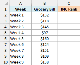
Below are the grocery bills for nine weeks, and I want to compare the PERCENTRANK.INC ranks in column C with the PERCENTRANK.EXC ranks in column D.
Here is the PERCENTRANK.INC formula for column C:
=PERCENTRANK.INC(B2:B10,B2:B10)
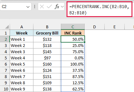
PERCENTRANK.INC gives the lowest bill ($97 in Week 4) 0% and the highest bill ($160 in Week 5) 100%. The other weeks are spread evenly between them, 12.5% apart.
And here is the PERCENTRANK.EXC formula for column D:
=PERCENTRANK.EXC(B2:B10,B2:B10)
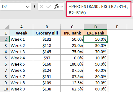
PERCENTRANK.EXC gives the same two weeks 10% and 90%, and the other weeks are 10% apart.
The difference comes from the math. INC divides the number of lower values by one less than the count (8 here), while EXC adds 1 to the number of lower values and divides by one more than the count (10 here).
Both put the middle bill ($132 in Week 1) at 50%. The gap between them is biggest at the two ends, and it gets smaller as your list gets longer.
If your report uses PERCENTILE.EXC to find percentile values, use PERCENTRANK.EXC for the ranks too. That way, both work on the same exclusive scale.
So these are a few ways you can use the PERCENTRANK.EXC function in Excel, from ranking a whole list to ranking a value within one group. I hope you found this tutorial helpful.
Other Excel Articles You May Also Like:
