

The HEX2OCT function in Excel converts a hexadecimal number (base 16, which uses 0 to 9 and A to F) into an octal number (base 8, which uses only 0 to 7). For example, it turns the hex number 1F into 37.
Hex and octal are both short ways of writing binary numbers, so you’ll mostly run into them in programming and other computer-related data. HEX2OCT lets you go from one to the other directly, without converting to decimal first.
HEX2OCT has two catches, though. It can’t take a range of cells directly (you need a small trick for that), and it stops working above the hex number 1FFFFFFF, even though it accepts up to 10 characters.
In this tutorial, I’ll show you how to convert a whole list at once, add leading zeros, handle the 0x prefix, convert negative numbers, get past the size limit, and fix the #NUM! error.
Follow along with the example file
HEX2OCT Function Examples.xlsx
HEX2OCT Function Syntax
Here is the syntax of the HEX2OCT function:
=HEX2OCT(number, [places])
- number – the hexadecimal number you want to convert. It can have up to 10 characters (0 to 9 and A to F, in upper or lower case), and can be text in double quotes, a number, or a cell reference. A 10-character number that starts with 8 to F is read as a negative number (Example 4 shows how this works).
- places – (optional) the number of characters you want in the result. HEX2OCT adds leading zeros to reach this length.
When you leave out places, HEX2OCT uses as few characters as it needs. So =HEX2OCT("1A") returns 32, while =HEX2OCT("1A",4) returns 0032.
If places is smaller than the result needs, you get a #NUM! error. For example, =HEX2OCT("FF",2) returns #NUM! because FF converts to 377, which needs three characters.
A places value of 0 or less also returns #NUM!, and text like “three” returns #VALUE!. A decimal value is cut down to a whole number, so 2.9 works like 2.
The HEX2OCT function works in Excel for Microsoft 365, Excel 2024, 2021, 2019, 2016, and Excel for Mac.
When to Use the HEX2OCT Function
Use this function when you need to:
- Convert hexadecimal numbers to octal without going through decimal first.
- Get octal codes of a fixed length, with leading zeros.
- Convert hex values copied from code, where they start with 0x.
- Convert negative hex numbers stored in 10-character form.
Let me show you a few practical examples of how to use the HEX2OCT function.
Example 1: Convert a List of Hex Numbers to Octal
Let’s start with a simple example.
Below is a list of hexadecimal numbers, and I want to convert each one to octal in column B.
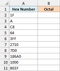
Here is the formula:
=HEX2OCT(+A2:A11)
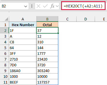
You enter this formula once in cell B2, and the results spill down to B11. HEX2OCT converts every hex number in A2:A11 to octal, so 1F becomes 37 and BEEF becomes 137357.
Important: Don’t skip the plus sign (+) before A2:A11. HEX2OCT can’t take a range reference directly, so =HEX2OCT(A2:A11) returns a single #VALUE! error instead of ten results.
The plus sign makes Excel read the values out of the range first and pass them to HEX2OCT as a list (an array), which it can work with.
HEX2OCT isn’t the only function like this, and here’s a look at other Excel functions that won’t spill on a range.
That article also mentions the double minus (--) and adding +0 as other ways to do the same thing. Don’t use those with HEX2OCT.
They try to turn each value into a regular number, and a hex number with a letter in it (like 1F or BEEF) can’t become one. So every such value returns #VALUE!, while the plus sign leaves the text as it is.
Also notice that the results sit on the left of the cells. That’s because HEX2OCT returns text, not a number, even when the result looks like one.
If you are using Excel 2019 or earlier, enter the below formula in cell B2 and then copy it down the range:
=HEX2OCT(A2)
This version doesn’t need the plus sign, because each formula points to just one cell. The same copy-down approach works for the other examples in this article.
Example 2: Get Fixed-Length Octal Codes With Leading Zeros
Now let’s use the places argument.
Every character you type has a code number, which the UNICODE function can give you in decimal. In programming, that code is often written in hex or in octal instead.
Below is a list of characters with their hex codes, and I want the octal code for each one in column C, always three digits long.
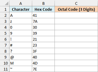
Here is the formula:
=HEX2OCT(+B2:B11,3)
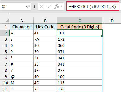
The 3 tells HEX2OCT to make every result three characters long, so it adds leading zeros where needed. For example, the hex code for the character 0 is 30, which converts to 60 and comes back as 060.
Codes that already have three digits stay as they are. The letter A has the hex code 41, which converts to 101.
Since HEX2OCT returns text, these leading zeros stay in the cell. A number like 060 would lose them, because Excel would show it as 60.
Three is enough for any two-digit hex code. The largest one, FF, converts to 377, which is three characters.
Example 3: Convert Hex Values That Start With 0x
In code and technical documents, hex numbers are often written with 0x in front (like 0x1F), so you can tell them apart from regular numbers. HEX2OCT doesn’t understand that prefix, so =HEX2OCT("0x1F") returns #NUM!.
Below is a list of hex values, most of them with the 0x prefix, and I want their octal versions in column B.
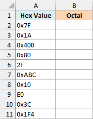
Here is the formula:
=HEX2OCT(SUBSTITUTE(A2:A11,"0x",""))
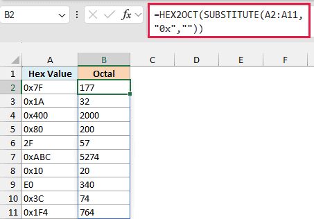
How this formula works:
- The SUBSTITUTE function replaces “0x” with nothing, so 0x7F becomes 7F. Values without the prefix, like 2F and E0, don’t have “0x” in them, so they stay as they are.
- HEX2OCT then converts the cleaned hex numbers to octal, so 7F becomes 177.
You don’t need the plus sign here, because the SUBSTITUTE function already hands HEX2OCT a list of values rather than a range reference.
The SUBSTITUTE function is case-sensitive, so a value written with a capital X (like 0X1F) keeps its prefix and returns #NUM!. If your data has both, use =HEX2OCT(SUBSTITUTE(UPPER(A2:A11),"0X","")) instead, which turns everything to upper case before removing the prefix.
Example 4: Convert Negative Hex Numbers With HEX2OCT
Now let’s look at negative numbers, which work a bit differently.
HEX2OCT reads a 10-character hex number that starts with 8 to F as a negative number. This is called two’s complement notation, and in it, FFFFFFFFFF is -1, FFFFFFFFFE is -2, and so on, counting down.
Below is a list of hex numbers along with the decimal value each one stands for, and I want their octal versions in column C, three characters long.
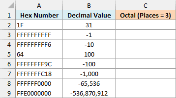
Here is the formula:
=HEX2OCT(+A2:A9,3)
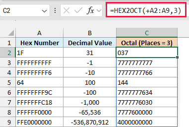
The positive numbers work the same way as in Example 2. 1F returns 037, and 64 returns 144.
The negative ones come back as 10-character octal numbers, even though I asked for three characters. For example, FFFFFFFFFF (which is -1) returns 7777777777.
A 10-character octal number that starts with 4 to 7 is negative, the same way a 10-character hex number that starts with 8 to F is. So trimming the leading digits would change the value.
That’s why HEX2OCT ignores places for negative numbers and always returns 10 characters.
For example, FFFFFFFF9C (which column B shows as -100) returns 7777777634. If you convert that back with the OCT2DEC function, =OCT2DEC("7777777634") returns -100 again.
The last row, FFE0000000 (-536,870,912), returns 4000000000. That’s the smallest negative number HEX2OCT can handle, so anything below it, like FFDFFFFFFF, returns #NUM!.
Important: A 10-character hex number that starts with 8 to F always comes back as negative (or #NUM!), even if you meant it as a positive number. For those, use the BASE and DECIMAL method in Example 5.
Example 5: Convert Hex Numbers Past HEX2OCT’s Limit
Let’s step it up with a case HEX2OCT can’t handle on its own.
HEX2OCT accepts up to 10 characters, but the largest positive number it converts is 1FFFFFFF (536,870,911 in decimal). That converts to 3777777777, and the next number up, 20000000, would give 4000000000.
As you saw in Example 4, a 10-character octal number that starts with 4 to 7 is negative (4000000000 is how HEX2OCT writes -536,870,912). So positive results have to stop at 3777777777.
Below is a list of hex numbers with 8 or 9 characters, and I want to try HEX2OCT in column B and then get the octal values with a method that works in column C.
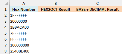
Here is the HEX2OCT formula:
=HEX2OCT(+A2:A8)
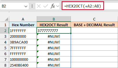
Only the first row works. 1FFFFFFF is right at the limit, and every number after it returns #NUM!, including 20000000, which is just one more.
Now here is the formula that works:
=BASE(DECIMAL(A2:A8,16),8)
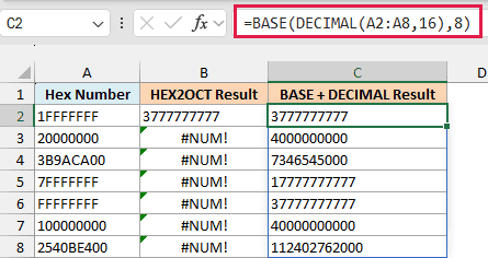
How this formula works:
- DECIMAL(A2:A8,16) converts each hex number to a regular decimal number. The 16 tells it the input is in base 16 (hex), so 3B9ACA00 becomes 1000000000.
- The BASE function then converts that decimal number to base 8, which is octal. So 1000000000 becomes 7346545000.
The DECIMAL function accepts a range directly, so this formula doesn’t need the plus sign. If you want leading zeros, the BASE function has its own third argument for the length, for example =BASE(DECIMAL(A2:A8,16),8,12).
This method works for hex numbers up to 1FFFFFFFFFFFFF (14 characters).
The BASE and DECIMAL functions treat every hex number as positive. So FFFFFFFFFF returns 17777777777777 with this method, while HEX2OCT reads it as -1 and returns 7777777777.
The BASE and DECIMAL functions are available in Excel 2013 and later versions.
Example 6: Why HEX2OCT Returns the #NUM! Error
Lastly, let’s look at what HEX2OCT does with inputs it can’t use.
Below are some inputs that commonly cause trouble, with a note on what’s in each cell, and I want to see what HEX2OCT returns for each one in column C.
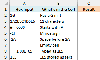
Here is the formula:
=HEX2OCT(+A2:A9)
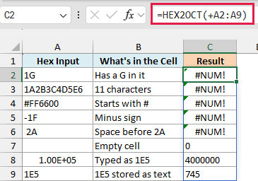
1G returns the #NUM! error because a hex number can only contain 0 to 9 and A to F. 1A2B3C4D5E6 returns #NUM! because it has 11 characters, one more than HEX2OCT allows.
#FF6600 and -1F return #NUM! too, because HEX2OCT doesn’t accept a # or a minus sign. You can remove the # with the SUBSTITUTE function, the same way as in Example 3, and negative numbers have to be in the 10-character form shown in Example 4.
The value in A6 has a space before 2A, which is easy to miss when you copy data from somewhere else. The TRIM function removes it, so =HEX2OCT(TRIM(A6)) returns 52.
An empty cell doesn’t return an error. HEX2OCT treats it as 0 and returns 0, which looks like a valid result, so make sure every input cell has a value.
The next row is the sneaky one. I typed 1E5 in cell A8, but Excel read it as scientific notation for 100000 and stored that number instead (which is why it shows as 1.00E+05).
HEX2OCT then reads the digits 100000 as a hex number and returns 4000000, without any error. The last row has 1E5 stored as text, and that gives the right result, 745.
Important: A hex number made of digits with a single E in between (like 1E5 or 3E8) turns into a regular number as soon as you type it. Format the cells as Text before typing, or start the entry with an apostrophe (‘1E5).
So these are a few examples of how to use the HEX2OCT function in Excel. Just keep the 1FFFFFFF limit in mind, and use the plus sign (not the double minus) when you convert a whole range at once.
If you need to go the other way, the OCT2HEX function converts octal back to hex. And if you need decimal or binary instead, Excel has the HEX2DEC and HEX2BIN functions.
Other Excel Articles You May Also Like:
