

Sometimes, you may want the options in one drop-down list to change based on what you pick in another. This is called a dependent drop-down list.
For example, when you pick Furniture as the category, the second drop-down should only show items such as Chairs and Tables.
Excel doesn’t have this as a built-in feature, but nothing to worry about. One formula inside the Data Validation dialog box can get this done.
In this article, I’ll show you how to create dependent drop-down lists using XLOOKUP, build multi-level lists, use the INDIRECT method, and fix wrong selections.
Follow along with the example file
Dependent Drop Down List in Excel.xlsx
What Is a Dependent Drop Down List in Excel?
An Excel drop-down list is a useful feature when you’re creating data entry forms or Excel Dashboards.
It shows a list of items in a cell, and you can pick one instead of typing it. This is handy when you often need to enter names, products, or regions in a set of cells.
Read: Here is a detailed guide on how to create an Excel Drop Down List.
Sometimes, however, you want a second drop-down list whose items depend on the selection made in the first drop-down list.
These are called dependent drop-down lists (also known as conditional drop-down lists).
Below is an example of what I mean:
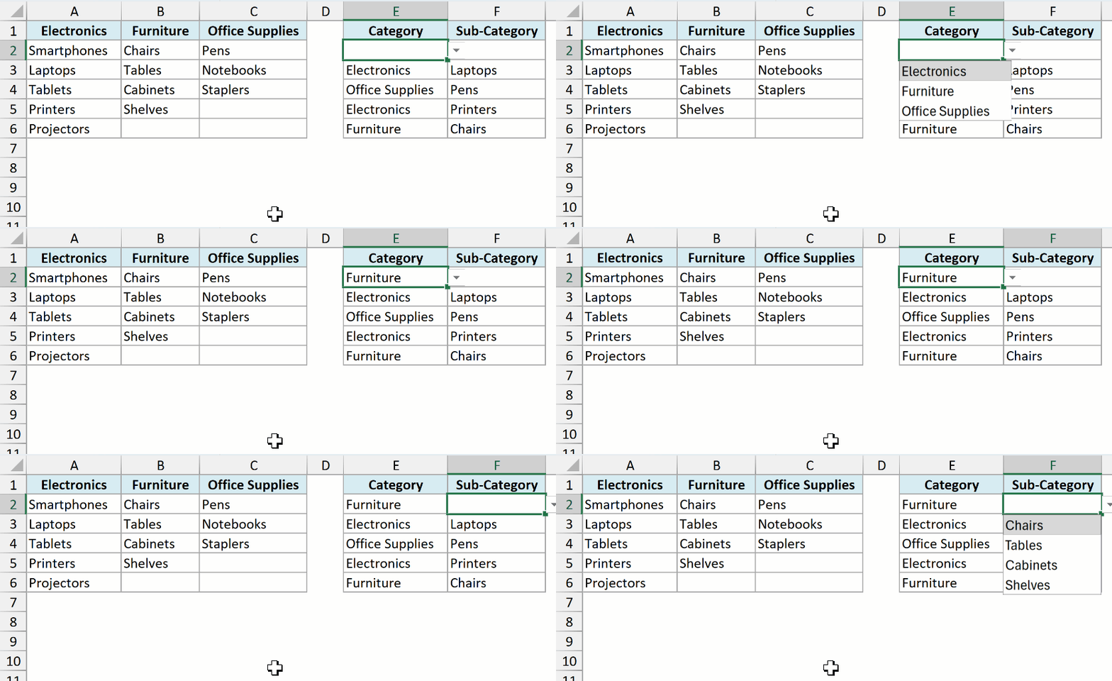
If I select Furniture as the Category, the Sub-Category drop-down shows only the furniture items. If I select Electronics, it shows only the electronics items.
Create a Dependent Drop Down List Using XLOOKUP (Without INDIRECT)
This is the method I recommend if you have Excel 2021, Excel 2024, or Microsoft 365.
It needs no named ranges, and it keeps working even when a category name has a space in it.
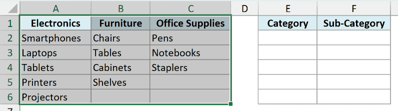
Below I have a dataset with three categories in A1:C1 and the items for each category below them.
I want a Category drop-down in E2:E6 and a dependent Sub-Category drop-down in F2:F6.
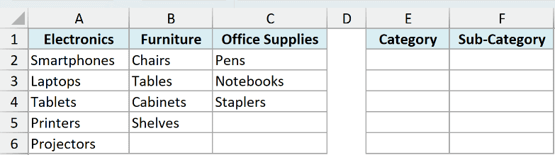
Let’s first create the Category drop-down. Here are the steps:
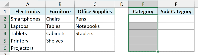
- Select the cells where you want the Category drop-down (E2:E6 in this example).
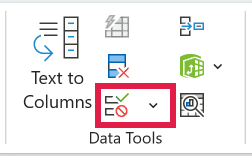
- Go to the Data tab, and in the Data Tools group, click on Data Validation. This opens the Data Validation dialog box.
Pro Tip: You can also open the Data Validation dialog box with the keyboard shortcut ALT + A + V + V on Windows (press these keys one after the other).
- In the Settings tab, select List in the Allow drop-down.
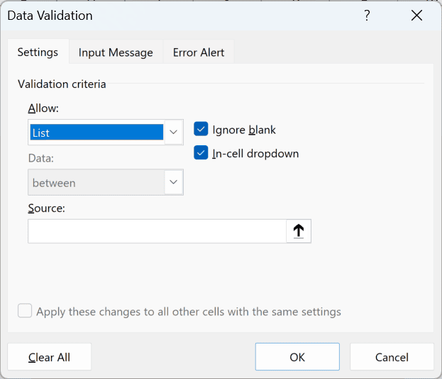
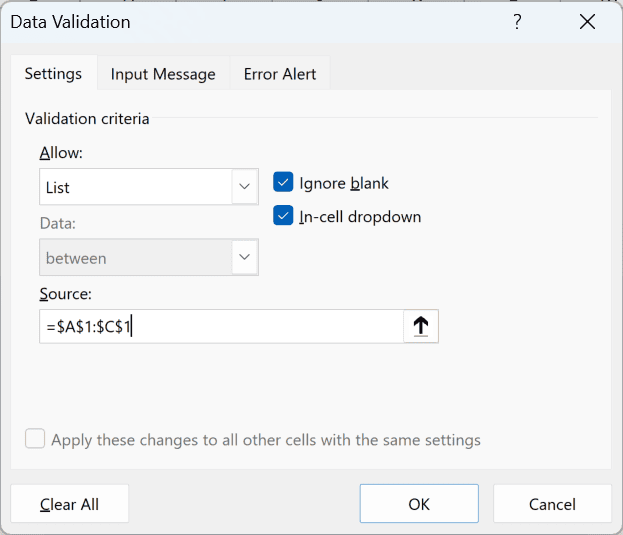
- In the Source field, enter =$A$1:$C$1 (or select the category names A1:C1 with your mouse).
- Click OK.
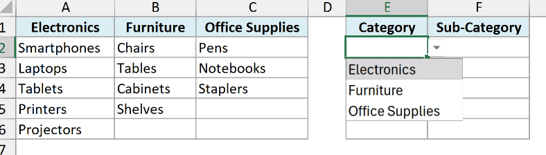
Now each cell in E2:E6 has a drop-down that shows Electronics, Furniture, and Office Supplies.
Next, let’s create the dependent Sub-Category drop-down. Here are the steps:
- Select the cells where you want the dependent drop-down (F2:F6 in this example).
- Open the Data Validation dialog box (Data tab, then Data Validation).
- Select List in the Allow drop-down.
- In the Source field, enter the formula below.
=XLOOKUP(E2,$A$1:$C$1,$A$2:$C$6)
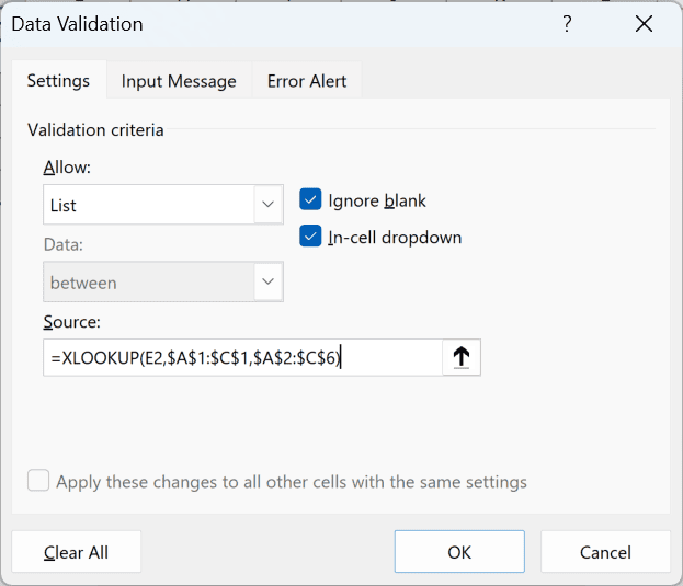
- Click OK.
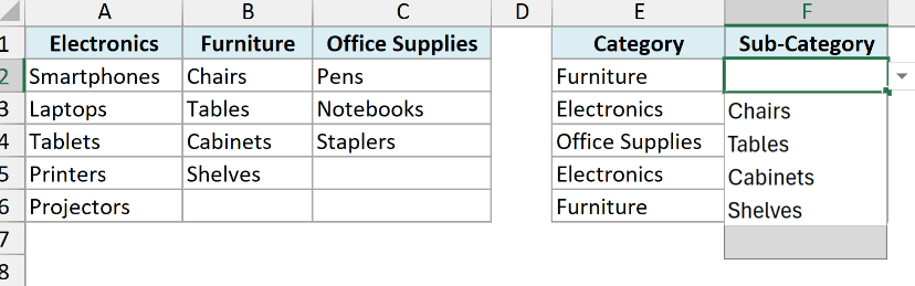
Important: If column E is still empty when you click OK, Excel warns that the Source currently evaluates to an error. Click Yes. The list works as soon as you pick a category.
Now, when you pick a category in column E, the drop-down in the same row of column F only shows the items for that category.
How this formula works:
- E2 – This is the category selected in the same row. It’s a relative reference, so row 3 looks at E3, row 4 looks at E4, and so on.
- $A$1:$C$1 – This is where XLOOKUP looks for the selected category.
- $A$2:$C$6 – This is the list of items. XLOOKUP returns the whole column below the matching category, and that column becomes the drop-down list.
Important: Make sure the ranges have dollar signs (absolute references) and E2 does not. Otherwise, the drop-downs in the rows below will look at the wrong cells.
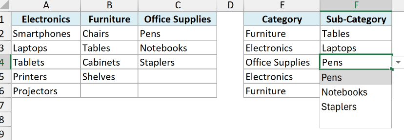
There is one small thing you’ll notice with this formula. Furniture has four items and Office Supplies has three, so their columns have empty cells at the bottom.
These empty cells show up as a blank option at the end of the drop-down (only one blank, even when there are multiple empty cells).
In most cases this is fine, but if it bothers you, the next section removes it.
Remove the Blank Option from the Dependent Drop Down
If you only want the actual items in the dependent drop-down and no blank at the end, you can wrap the XLOOKUP formula in the TAKE function.
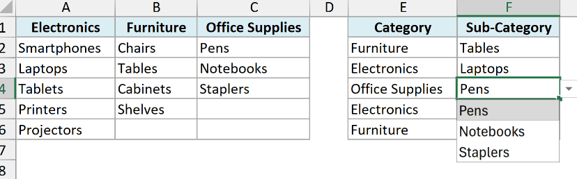
Below is the same setup from the previous section. When Office Supplies is selected in E4, the drop-down in F4 shows its three items plus a blank at the end.
Here are the steps to update the dependent drop-down:
- Select F2:F6 and open the Data Validation dialog box.
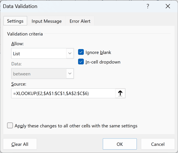
- In the Source field, replace the existing formula with the formula below, and click OK.
=TAKE(XLOOKUP(E2,$A$1:$C$1,$A$2:$C$6),COUNTIF(XLOOKUP(E2,$A$1:$C$1,$A$2:$C$6),"?*"))
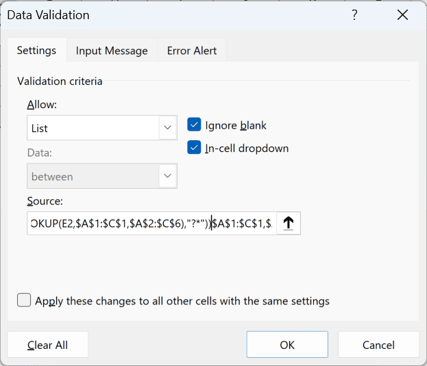
Now, when you select Office Supplies in column E, the drop-down in column F shows only Pens, Notebooks, and Staplers, with no blank at the end.
How this formula works:
- XLOOKUP(E2,$A$1:$C$1,$A$2:$C$6) – This returns the full column of items for the selected category, including the empty cells at the bottom.
- COUNTIF(…,”?“) – This counts how many cells in that column have text. The “?” criteria means at least one character, so empty cells are not counted.
- TAKE(…) – TAKE keeps only that many cells from the top of the list, which drops the empty cells at the bottom.
Note that this formula expects the items in each column to be text with no gaps in between.
An item typed as a number (such as 12) is not counted by “?*”, and an empty cell in the middle of a list would cut the list short.
Important: The TAKE function is only available in Microsoft 365 and Excel 2024. In Excel 2021, use the plain XLOOKUP formula from the previous section.
Follow along with the example file
Dependent Drop Down List in Excel.xlsx
Multi-Level Dependent Drop Down List (Category, Sub-Category, Product)
The same idea can be extended to create multiple dependent drop-down lists, where each drop-down depends on the one before it.
Below I have a dataset where column A has the Category, column B has the Sub-Category, column C has the Product, and column D has the Price.
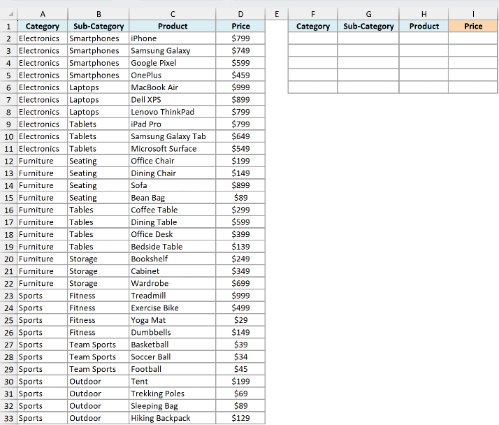
I want a Category drop-down in column F, a Sub-Category drop-down in column G that depends on the category, and a Product drop-down in column H that depends on the sub-category.
Important: This method only works when the data is sorted, so all the rows for one category sit together, and so do all the rows for one sub-category. If your data isn’t sorted, sort it first.
Let’s start with the Category drop-down:
- Select F2:F6 and open the Data Validation dialog box.
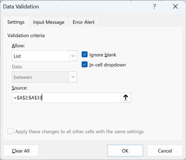
- Select List, enter =$A$2:$A$33 in the Source field, and click OK.
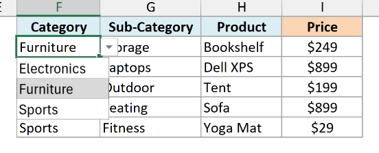
Column A has each category repeated many times, but the drop-down shows Electronics, Furniture, and Sports only once each.
Note that this is how the latest version of Excel in Microsoft 365 works. Older versions of Excel may show the duplicates in the drop-down list.
Now let’s create the Sub-Category drop-down. Select G2:G6, open the Data Validation dialog box, select List, and enter this formula in the Source field:
=DROP(TAKE($B$2:$B$33,XMATCH(F2,$A$2:$A$33,0,-1)),XMATCH(F2,$A$2:$A$33)-1)
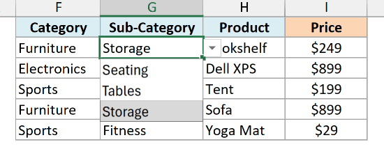
When Furniture is selected in F2, the Sub-Category drop-down in G2 shows Seating, Tables, and Storage. If Excel warns that the Source evaluates to an error when you click OK, click Yes.
How this formula works:
- XMATCH(F2,$A$2:$A$33) – This finds the first position of the selected category in column A. For Furniture, it’s 11.
- XMATCH(F2,$A$2:$A$33,0,-1) – The -1 tells XMATCH to search from the bottom, so this finds the last position of Furniture, which is 21.
- TAKE($B$2:$B$33,21) – This keeps the first 21 sub-categories, so everything after the last Furniture row is gone.
- DROP(…,11-1) – This removes the first 10 rows, so only the Furniture rows (positions 11 to 21) are left.
The Furniture rows repeat Seating, Tables, and Storage several times, but just like the category list, each one shows up only once in the drop-down.
The Product drop-down uses the exact same logic, just shifted one column to the right. Select H2:H6, open the Data Validation dialog box, select List, and use this formula:
=DROP(TAKE($C$2:$C$33,XMATCH(G2,$B$2:$B$33,0,-1)),XMATCH(G2,$B$2:$B$33)-1)
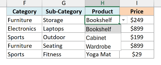
When Storage is selected in G2, the Product drop-down in H2 shows Bookshelf, Cabinet, and Wardrobe.
Note that this formula searches the whole Sub-Category column, so each sub-category name should appear under only one category.
If two categories have a sub-category with the same name, rename one of them.
You can keep extending this logic for as many levels as your data has.
And since every product name is unique, you don’t need another drop-down for the price. A simple XLOOKUP formula in I2 (copied down) fetches it:
=XLOOKUP(H2,$C$2:$C$33,$D$2:$D$33,"")
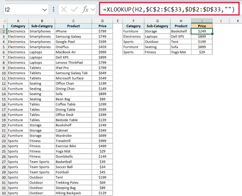
This returns $249 for the Bookshelf in H2. The “” at the end returns a blank instead of an error when no product is selected in that row.
Important: TAKE and DROP are only available in Microsoft 365 and Excel 2024, and XMATCH needs Excel 2021 or later.
Also read: Creating a Drop Down Filter to Extract Data Based on Selection
Dependent Drop Down List Using INDIRECT and Named Ranges
If you’re using an older version of Excel (such as Excel 2019 or 2016), you can create a dependent drop-down list using named ranges and the INDIRECT function.
This is also the method to use when you need to share the file with someone on an older version.
Below I have the same dataset, with three categories in A1:C1 and the items for each category below them.
I want a Category drop-down in E2:E6 and a dependent drop-down in F2:F6.
Here are the steps to create a dependent drop-down list using INDIRECT:
- Select E2:E6, go to Data, then Data Validation, select List, enter =$A$1:$C$1 in the Source field, and click OK. This creates the Category drop-down.
- Select the entire dataset (A1:C6 in this example).
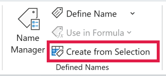
- Go to Formulas, then Defined Names, then Create from Selection (or use the keyboard shortcut Control + Shift + F3).
- In the Create Names from Selection dialog box, check the Top row option, uncheck all the others, and click OK.
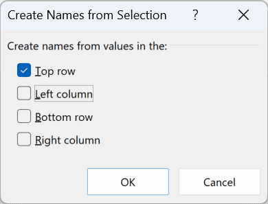
This creates three named ranges (Electronics, Furniture, and Office_Supplies), where each name refers to the items below that category.
- Select the cells where you want the dependent drop-down (F2:F6 in this example).
- Open the Data Validation dialog box, and in the Settings tab, make sure List is selected.
- In the Source field, enter the formula below, and click OK.
=INDIRECT(SUBSTITUTE(E2," ","_"))
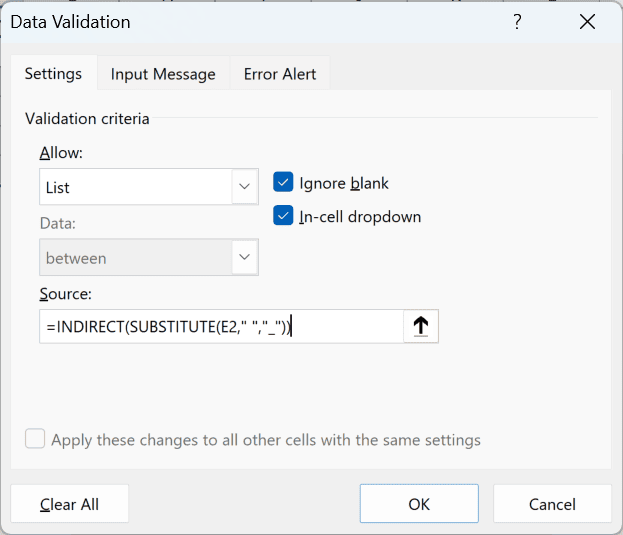
If column E is still empty, Excel warns that the Source currently evaluates to an error. Click Yes, as the list works once a category is picked.
Now, when you make a selection in the Category drop-down, the options in the dependent drop-down automatically update.
How does this work?
When you select Furniture in E2, the INDIRECT function turns that text into a reference to the named range Furniture, so the drop-down lists all the furniture items.
The reason for the SUBSTITUTE function is that Excel does not allow spaces in named ranges.
So when you create a named range from a two-word heading like Office Supplies, Excel names it Office_Supplies.
SUBSTITUTE converts the space in E2 into an underscore so INDIRECT finds the right name.
If none of your categories have a space in them, the simpler formula =INDIRECT(E2) works as well.
Note that the named ranges cover rows 2 to 6 for every category, so shorter lists (such as Office Supplies) show a blank option at the end of the drop-down.
Also, if you rename a category heading later, you need to create the names again.
Follow along with the example file
Dependent Drop Down List in Excel.xlsx
Highlight Wrong Selections in the Dependent Drop Down
There is one problem with all the methods above.
When you change the first drop-down after making a selection in the dependent drop-down, the dependent drop-down does not change.
For example, if you select Furniture as the category and Chairs as the sub-category, and then go back and change the category to Electronics, the sub-category still shows Chairs.
A simple conditional formatting rule can highlight the cell whenever there is a mismatch, so you can see it and correct it.
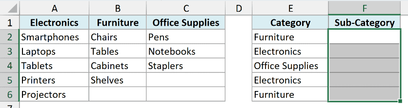
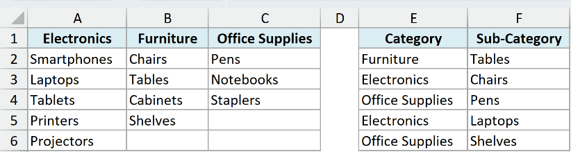
Below I have a dataset with categories in A1:C1, the Category drop-down in E2:E6, and the dependent Sub-Category drop-down in F2:F6.
Rows 3 and 6 have a sub-category that doesn’t belong to the category.
Here are the steps to highlight mismatches in the dependent drop-down list:
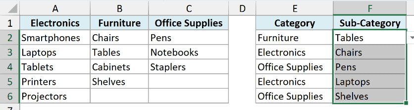
- Select the cells that have the dependent drop-down list (F2:F6 in this example).
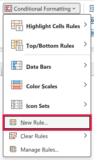
- Go to Home, then Conditional Formatting, then New Rule.
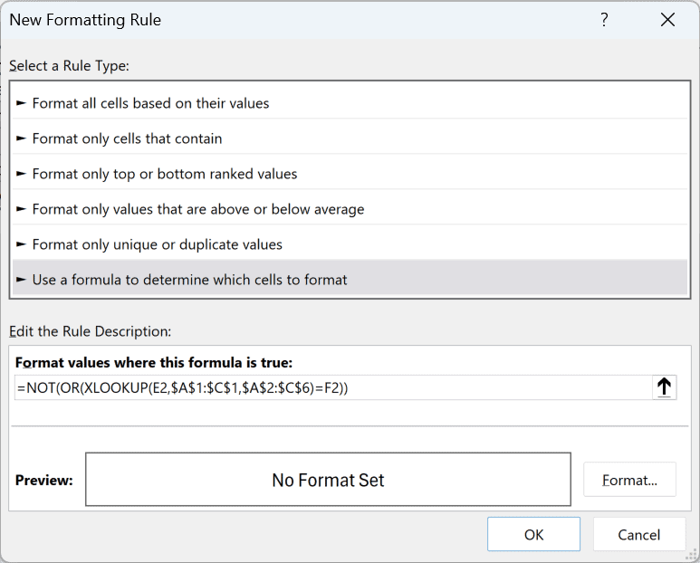
- In the New Formatting Rule dialog box, select ‘Use a formula to determine which cells to format’.
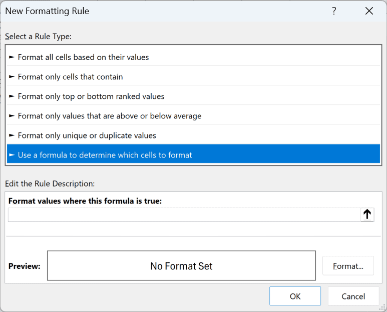
- In the formula field, enter the formula below.
=NOT(OR(XLOOKUP(E2,$A$1:$C$1,$A$2:$C$6)=F2))
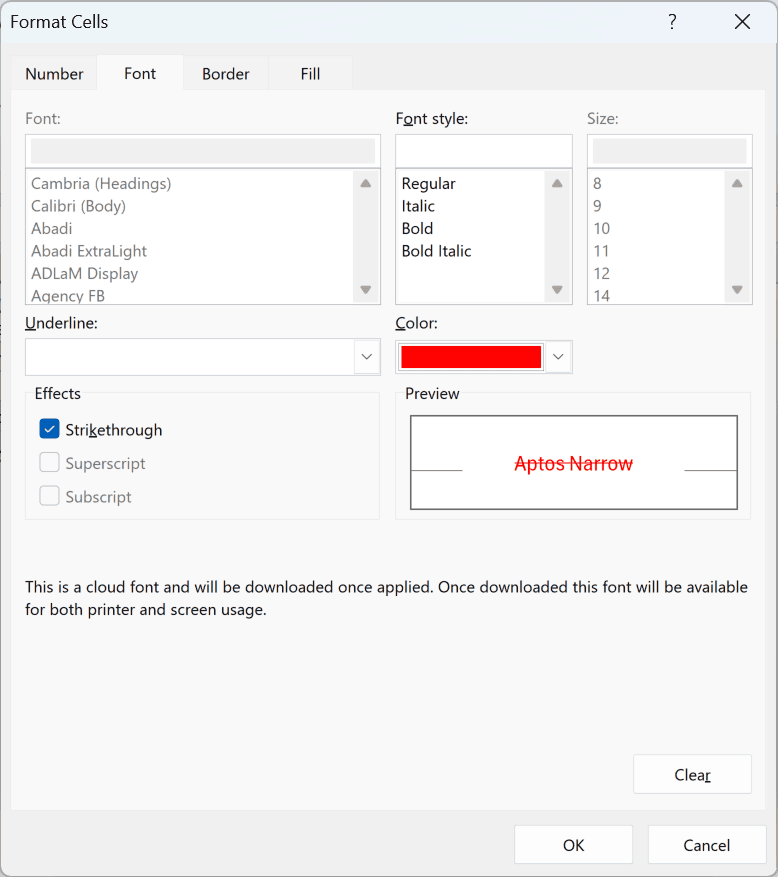
- Click the Format button, and in the Font tab, check Strikethrough and set the Color to red.
- Click OK, and then click OK again.
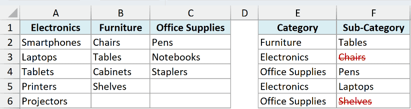
Now Chairs (under Electronics) and Shelves (under Office Supplies) show in red with a strikethrough. As soon as you pick a valid sub-category, the formatting goes away.
How this formula works:
- XLOOKUP(E2,$A$1:$C$1,$A$2:$C$6) – This returns all the items for the category selected in E2.
- …=F2 – This compares each of those items with the value in F2 and gives a TRUE for a match and FALSE otherwise.
- OR(…) – This returns TRUE if any one of them matched, which means the selection is valid.
- NOT(…) – This flips the result, so a mismatch returns TRUE, and that tells conditional formatting to format the cell.
Note that this rule highlights the wrong selection but does not change it. The old value stays in the cell until you pick a new one.
Also, since this rule uses XLOOKUP, it needs Excel 2021 or later. If you’re on Excel 2019 or earlier, use this formula in the same rule instead:
=ISERROR(VLOOKUP(F2,INDEX($A$2:$C$6,,MATCH(E2,$A$1:$C$1,0)),1,0))
MATCH finds the column of the selected category, and INDEX returns that column of items. The VLOOKUP function then looks for F2 in it.
If F2 is not in that column, VLOOKUP returns an error, and ISERROR turns that into TRUE, which tells conditional formatting to highlight the cell.
You can see this rule on the INDIRECT Method sheet in the example file.
Show “Please Select” Instead of the Wrong Selection
Instead of highlighting a wrong selection, you can make it disappear and show a message such as Please select in its place.
This uses the same formula, with a custom number format instead of a strikethrough.
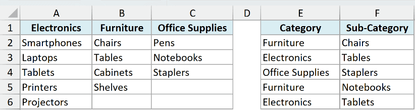
Below I have the same setup, with the Category drop-down in E2:E6 and the dependent drop-down in F2:F6. Rows 3 and 5 have a sub-category that doesn’t belong to the category.
Here are the steps:
- Select F2:F6, go to Home, then Conditional Formatting, then New Rule.
- Select ‘Use a formula to determine which cells to format’, and enter =NOT(OR(XLOOKUP(E2,$A$1:$C$1,$A$2:$C$6)=F2)) in the formula field.
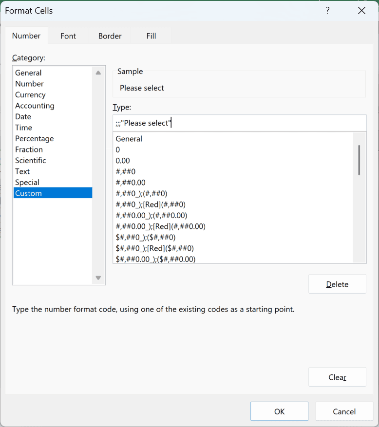
- Click Format, and in the Number tab, select Custom and enter ;;;”Please select” in the Type field.
- Go to the Font tab, set the Color to red, and click OK twice.
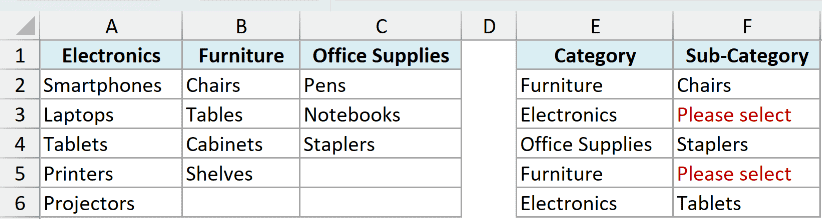
Now F3 and F5 show Please select in red, and they go back to normal as soon as you pick a valid sub-category.
A custom number format has four parts separated by semicolons: positive numbers, negative numbers, zeros, and text.
By leaving the first three empty and putting “Please select” in the text part, any text in the cell displays as Please select.
Important: The wrong value is still in the cell. You can see it in the formula bar, and any formula that refers to this cell still uses it.
Clear the Dependent Drop Down Automatically Using VBA
If you want the dependent drop-down to actually reset whenever the main drop-down changes, you need VBA.
I personally prefer the conditional formatting method, because VBA code needs a macro-enabled file, and the person you share it with has to enable macros.
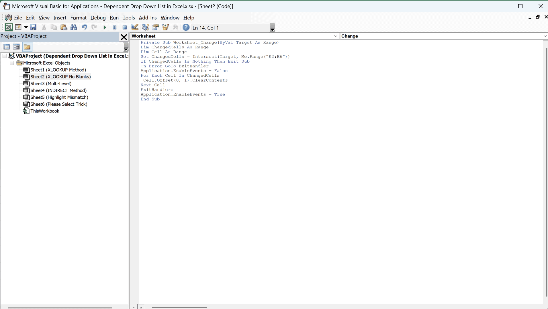
Here is the VBA code to clear the contents of a dependent drop-down list:
Private Sub Worksheet_Change(ByVal Target As Range)
Dim ChangedCells As Range
Dim Cell As Range
Set ChangedCells = Intersect(Target, Me.Range("E2:E6"))
If ChangedCells Is Nothing Then Exit Sub
On Error GoTo ExitHandler
Application.EnableEvents = False
For Each Cell In ChangedCells
 Cell.Offset(0, 1).ClearContents
Next Cell
ExitHandler:
Application.EnableEvents = True
End SubThis code uses the Worksheet_Change event, so it runs whenever a cell changes on the sheet.
If the changed cells are in E2:E6 (where the Category drop-downs are), it clears the cell to the right of each one (the dependent drop-down). Changes anywhere else on the sheet are ignored.
If your main drop-downs are in a different range, change E2:E6 in the code to that range.
This code is based on this tutorial by Debra on clearing dependent drop down lists in Excel when the selection is changed.
Here is how to make this code work:
- Copy the VBA code.
- In the workbook that has the dependent drop-down list, go to the Developer tab, and in the Code group, click on Visual Basic (or use the keyboard shortcut ALT + F11).

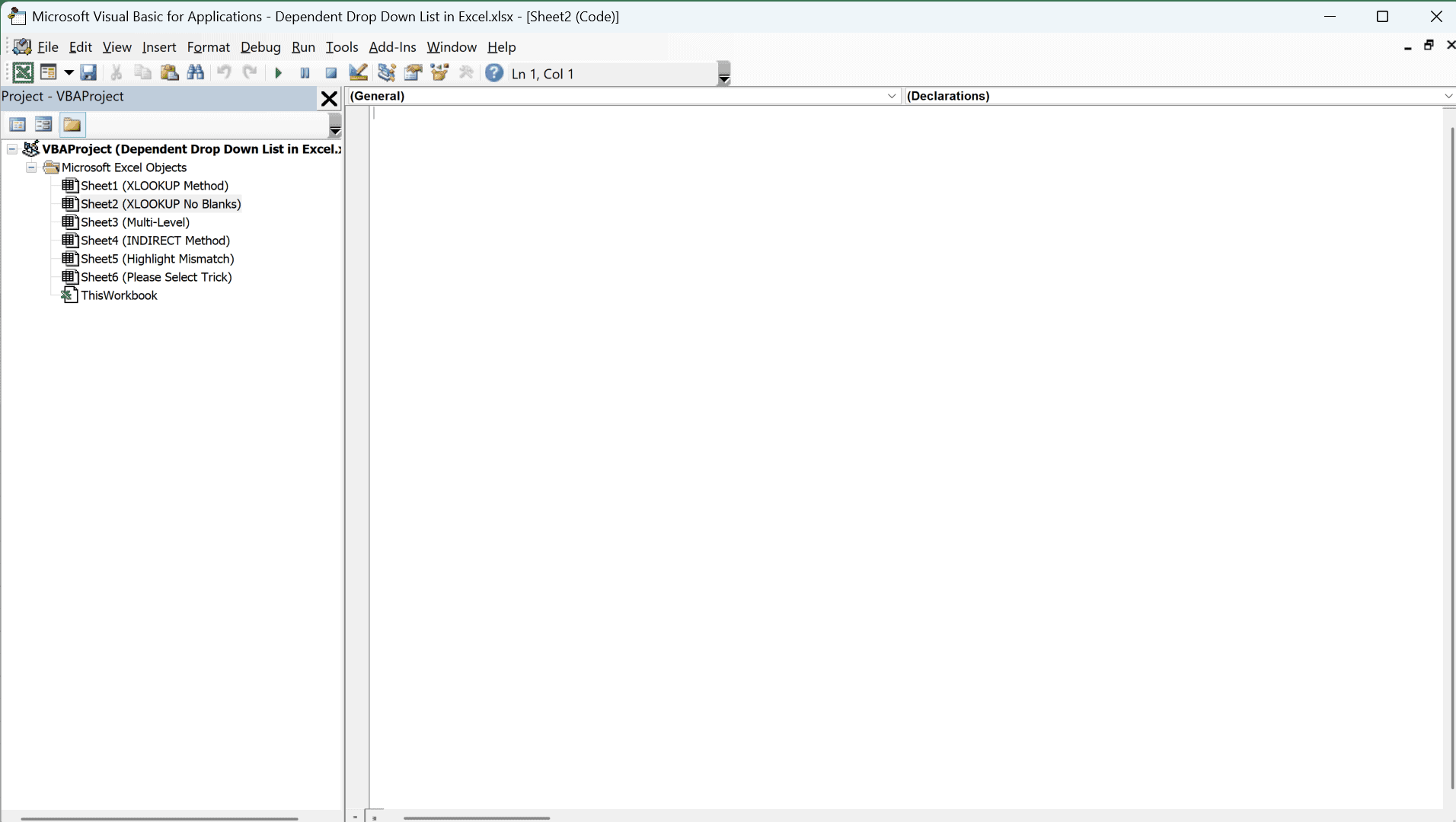
- In the Project Explorer on the left, you’ll see all the worksheet names. Double-click on the sheet that has the drop-down list.
- Paste the code in the code window on the right.
- Close the VB Editor.
Now, whenever you change the main drop-down, the code clears the dependent drop-down next to it.
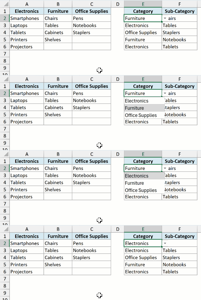
If you’d rather show a message than an empty cell, replace the ClearContents line with Cell.Offset(0, 1).Value = “— Make Selection —“.
Important: Save the file as a macro-enabled workbook (.xlsm). If you save it as a regular .xlsx file, the code is removed.
Also note that you can’t undo a change made by VBA, so the cleared value can’t be brought back with Control + Z.
So these are the ways you can create a dependent drop-down list in Excel, along with a few ways to handle wrong selections when the first drop-down changes.
I hope you found this Excel tutorial useful.
Other Excel Articles You May Also Like:
- Extract Data based on a drop-down list selection
- Creating a drop-down list with search suggestions
- Select multiple items from a drop-down list
- Create multiple drop-down lists without repetition
- Save Time with Data Entry Forms in Excel
- Create Data Validation List from Excel Table as Source
- Display Main and Subcategory in Drop Down List in Excel
- How to Make a Yes/No Drop-Down in Excel
- Enable Conditional Data Entry in Excel using Data Validation

Thanks, this was awesome.
Much simpler than many ways I’ve seen.
A little side note:
The formula won’t work if the name isn’t exakt.
I, for instance, used “:” after my titles. Which couldn’t be picked up by the name manager, and thus it didn’t work, until I removed the colon.
Is it also possible to rewrite the formula to apply on whole column ? E.g. in column A I select Vegetable and in column B I will get a drop-down with valid vegetable values. If I change Vegetable value in A to Fruit I would get a drop-down for fruit.
The expanding the data validation pattern cell by cell in excel is not a solution for me as I’m generating the excel file and not creating it manually.
Thank you very much for the video!! what I am trying to do is when you select “India” all the names automatically go down in the column without you selecting one name if you select US all the names in the list will be copies in the column. How can i do it. I have 3 supervisors each have 14 team members under their name and they have to fill out a log. I don’t want them to click 14 times to get their team on the log. Can you please help me. thank you.
You should instead use the if command. Set each cell below to check if supervisor A is selected in that cell, then set the rest of the cells to fill a certain name. Each cell would be set to only one name per supervisor.
This is great, but I have a problem. My Column headers are 2 words and not a single word like “Fruit” or “Vegetable” but rather “Fruit and Vegetable” and “Grains and Breads.” I require a 2 word header value/name. The “named range” uses underscore (_) between each word, which is fine, but the secondary/dependent drop-down does not populate.
thanks for any tips or advice on a workaround of this nature.
Is it possible to put the data in another worksheet of the same excel and use the indirect function?