

Sometimes, you may want the options in one drop-down list to change based on what you pick in another. This is called a dependent drop-down list.
For example, when you pick Furniture as the category, the second drop-down should only show items such as Chairs and Tables.
Excel doesn’t have this as a built-in feature, but nothing to worry about. One formula inside the Data Validation dialog box can get this done.
In this article, I’ll show you how to create dependent drop-down lists using XLOOKUP, build multi-level lists, use the INDIRECT method, and fix wrong selections.
Follow along with the example file
Dependent Drop Down List in Excel.xlsx
What Is a Dependent Drop Down List in Excel?
An Excel drop-down list is a useful feature when you’re creating data entry forms or Excel Dashboards.
It shows a list of items in a cell, and you can pick one instead of typing it. This is handy when you often need to enter names, products, or regions in a set of cells.
Read: Here is a detailed guide on how to create an Excel Drop Down List.
Sometimes, however, you want a second drop-down list whose items depend on the selection made in the first drop-down list.
These are called dependent drop-down lists (also known as conditional drop-down lists).
Below is an example of what I mean:
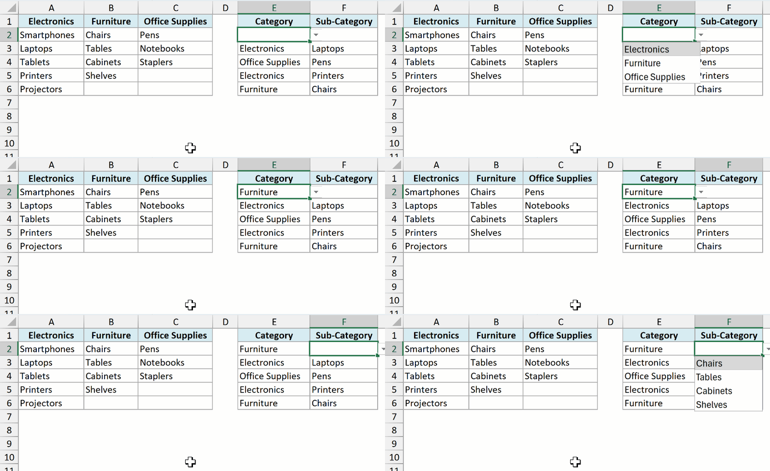
If I select Furniture as the Category, the Sub-Category drop-down shows only the furniture items. If I select Electronics, it shows only the electronics items.
Create a Dependent Drop Down List Using XLOOKUP (Without INDIRECT)
This is the method I recommend if you have Excel 2021, Excel 2024, or Microsoft 365.
It needs no named ranges, and it keeps working even when a category name has a space in it.
Below I have items grouped into three categories, and I want a Category drop-down in column E and a dependent Sub-Category drop-down in column F.
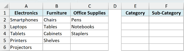
Let’s first create the Category drop-down. Here are the steps:
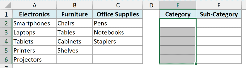
- Select the cells where you want the Category drop-down (E2:E6 in this example).
- Go to the Data tab, and in the Data Tools group, click on Data Validation. This opens the Data Validation dialog box.
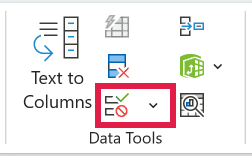
Pro Tip: You can also open the Data Validation dialog box with the keyboard shortcut ALT + A + V + V on Windows (press these keys one after the other).
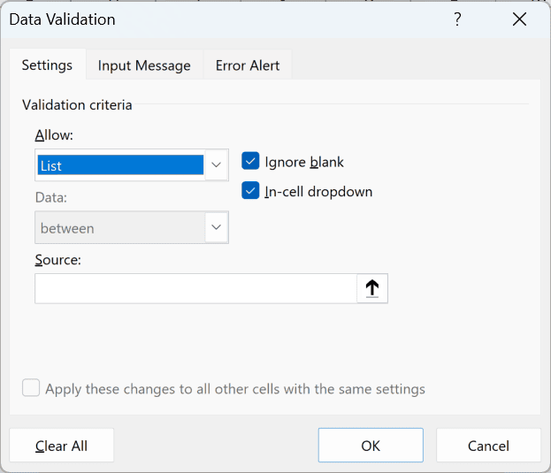
- In the Settings tab, select List in the Allow drop-down.
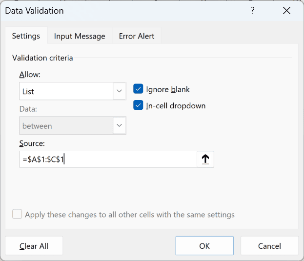
- In the Source field, enter =$A$1:$C$1 (or select the category names A1:C1 with your mouse).
- Click OK.
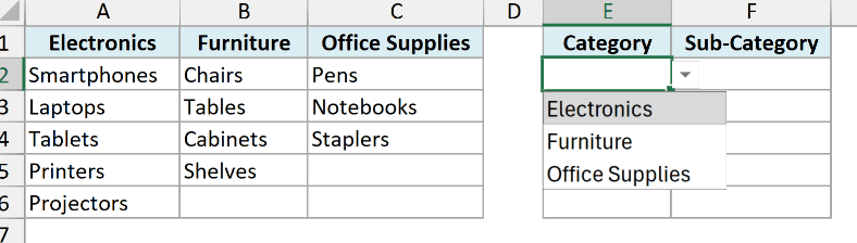
Now each cell in E2:E6 has a drop-down that shows Electronics, Furniture, and Office Supplies.
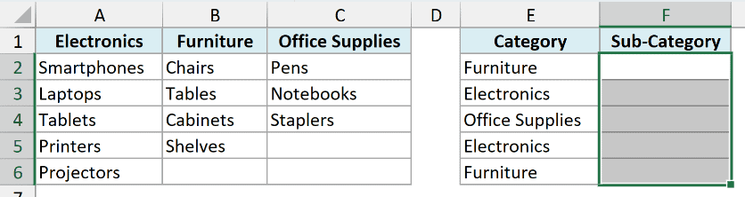
Next, let’s create the dependent Sub-Category drop-down. Here are the steps:
- Select the cells where you want the dependent drop-down (F2:F6 in this example).
- Open the Data Validation dialog box (Data tab, then Data Validation).
- Select List in the Allow drop-down.
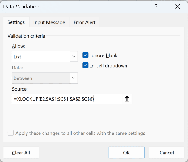
- In the Source field, enter the formula below.
=XLOOKUP(E2,$A$1:$C$1,$A$2:$C$6)
- Click OK.
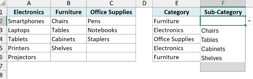
Important: If column E is still empty when you click OK, Excel warns that the Source currently evaluates to an error. Click Yes. The list works as soon as you pick a category.
Now, when you pick a category in column E, the drop-down in the same row of column F only shows the items for that category.
How this formula works:
- E2 – This is the category selected in the same row. It’s a relative reference, so row 3 looks at E3, row 4 looks at E4, and so on.
- $A$1:$C$1 – This is where XLOOKUP looks for the selected category.
- $A$2:$C$6 – This is the list of items. XLOOKUP returns the whole column below the matching category, and that column becomes the drop-down list.
Important: Make sure the ranges have dollar signs (absolute references) and E2 does not. Otherwise, the drop-downs in the rows below will look at the wrong cells.
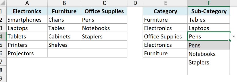
There is one small thing you’ll notice with this formula. Furniture has four items and Office Supplies has three, so their columns have empty cells at the bottom.
These empty cells show up as a blank option at the end of the drop-down (only one blank, even when there are multiple empty cells).
In most cases this is fine, but if it bothers you, the next section removes it.
Remove the Blank Option from the Dependent Drop Down
If you only want the actual items in the dependent drop-down and no blank at the end, you can wrap the XLOOKUP formula in the TAKE function.
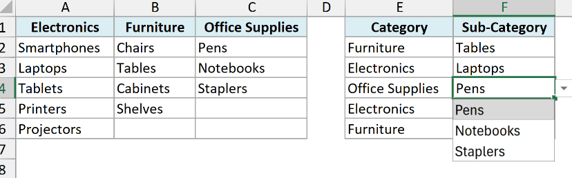
Below is the same setup from the previous section. When Office Supplies is selected in E4, the drop-down in F4 shows its three items plus a blank at the end.
Here are the steps to update the dependent drop-down:
- Select F2:F6 and open the Data Validation dialog box.
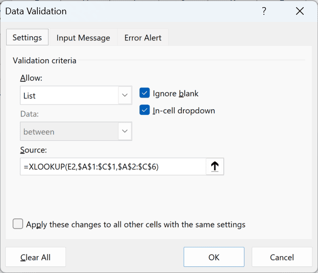
- In the Source field, replace the existing formula with the formula below, and click OK.
=TAKE(XLOOKUP(E2,$A$1:$C$1,$A$2:$C$6),COUNTIF(XLOOKUP(E2,$A$1:$C$1,$A$2:$C$6),"?*"))
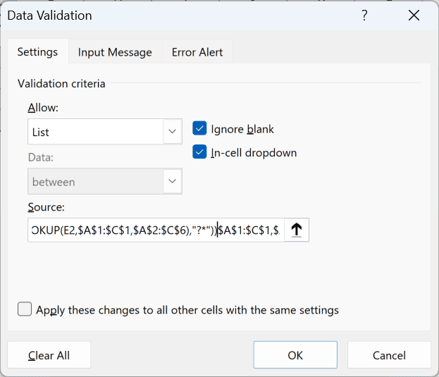
Now, when you select Office Supplies in column E, the drop-down in column F shows only Pens, Notebooks, and Staplers, with no blank at the end.
How this formula works:
- XLOOKUP(E2,$A$1:$C$1,$A$2:$C$6) – This returns the full column of items for the selected category, including the empty cells at the bottom.
- COUNTIF
(...,"?*")– This counts how many cells in that column have text. The"?*"criteria means at least one character, so empty cells are not counted. - TAKE(…) – TAKE keeps only that many cells from the top of the list, which drops the empty cells at the bottom.
The COUNTIF function uses “?*” to count text, so an item typed as a number (such as 12) isn’t counted. Make sure each item is stored as text.
Also, an empty cell in the middle of a list would cut the list short, so keep all the items together with no gaps.
Important: The TAKE function is only available in Microsoft 365 and Excel 2024. In Excel 2021, use the plain XLOOKUP formula from the previous section.
Follow along with the example file
Dependent Drop Down List in Excel.xlsx
Multi-Level Dependent Drop Down List (Category, Sub-Category, Product)
The same idea can be extended to create multiple dependent drop-down lists, where each drop-down depends on the one before it.
Below I have products with categories, sub-categories, and prices, and I want linked Category, Sub-Category, and Product drop-downs in columns F, G, and H.
Each Sub-Category list depends on the category, and each Product list depends on the sub-category.
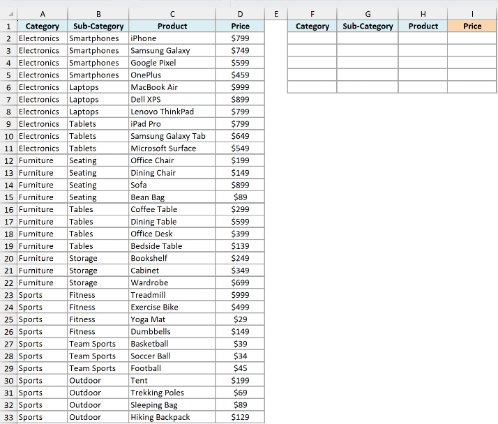
Important: This method only works when the data is sorted, so all the rows for one category sit together, and so do all the rows for one sub-category. If your data isn’t sorted, sort it first.
Let’s start with the Category drop-down:
- Select F2:F6 and open the Data Validation dialog box.
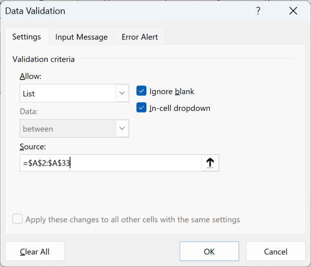
- Select List, enter =$A$2:$A$33 in the Source field, and click OK.
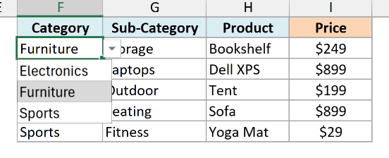
Column A has each category repeated many times, but the drop-down shows Electronics, Furniture, and Sports only once each.
Note that this is how the latest version of Excel in Microsoft 365 works. Older versions of Excel may show the duplicates in the drop-down list.
Now let’s create the Sub-Category drop-down. Select G2:G6, open the Data Validation dialog box, select List, and enter this formula in the Source field:
=DROP(TAKE($B$2:$B$33,XMATCH(F2,$A$2:$A$33,0,-1)),XMATCH(F2,$A$2:$A$33)-1)
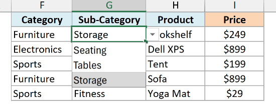
When Furniture is selected in F2, the Sub-Category drop-down in G2 shows Seating, Tables, and Storage.
If Excel warns that the Source evaluates to an error when you click OK, click Yes.
How this formula works:
- XMATCH(F2,$A$2:$A$33) – This finds the first position of the selected category in column A. For Furniture, it’s 11.
- XMATCH(F2,$A$2:$A$33,0,-1) – The -1 tells XMATCH to search from the bottom, so this finds the last position of Furniture, which is 21.
- TAKE($B$2:$B$33,21) – This keeps the first 21 sub-categories, so everything after the last Furniture row is gone.
- DROP(…,11-1) – This removes the first 10 rows, so only the Furniture rows (positions 11 to 21) are left.
The Furniture rows repeat Seating, Tables, and Storage several times, but just like the category list, each one shows up only once in the drop-down.
The Product drop-down uses the exact same logic, just shifted one column to the right. Select H2:H6, open the Data Validation dialog box, select List, and use this formula:
=DROP(TAKE($C$2:$C$33,XMATCH(G2,$B$2:$B$33,0,-1)),XMATCH(G2,$B$2:$B$33)-1)
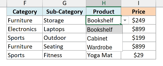
When Storage is selected in G2, the Product drop-down in H2 shows Bookshelf, Cabinet, and Wardrobe.
Note that this formula searches the whole Sub-Category column, so each sub-category name should appear under only one category.
If two categories have a sub-category with the same name, rename one of them.
You can keep extending this logic for as many levels as your data has.
And since every product name is unique, you don’t need another drop-down for the price. A simple XLOOKUP formula in I2 (copied down) fetches it:
=XLOOKUP(H2,$C$2:$C$33,$D$2:$D$33,"")
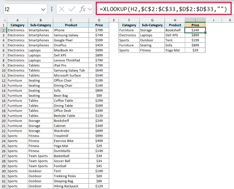
This returns $249 for the Bookshelf in H2. The “” at the end returns a blank instead of an error when no product is selected in that row.
Important: TAKE and DROP are only available in Microsoft 365 and Excel 2024, and XMATCH needs Excel 2021 or later.
Also read: Creating a Drop Down Filter to Extract Data Based on Selection
Dependent Drop Down List Using INDIRECT and Named Ranges
If you’re using an older version of Excel (such as Excel 2019 or 2016), you can create a dependent drop-down list using named ranges and the INDIRECT function.
This is also the method to use when you need to share the file with someone on an older version.
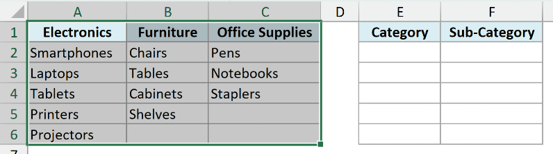
Below I have the same items grouped into three categories, and I want a Category drop-down in column E and a dependent drop-down in column F.
Here are the steps to create a dependent drop-down list using INDIRECT:
- Select E2:E6, go to Data, then Data Validation, select List, enter =$A$1:$C$1 in the Source field, and click OK. This creates the Category drop-down.
- Select the entire dataset (A1:C6 in this example).
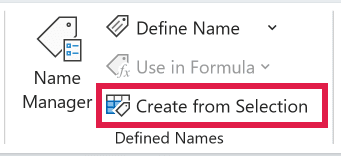
- Go to Formulas, then Defined Names, then Create from Selection (or use the keyboard shortcut Control + Shift + F3).
- In the Create Names from Selection dialog box, check the Top row option, uncheck all the others, and click OK.
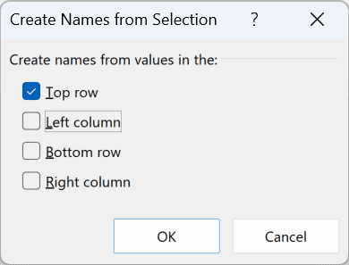
This creates three named ranges (Electronics, Furniture, and Office_Supplies), where each name refers to the items below that category.
- Select the cells where you want the dependent drop-down (F2:F6 in this example).
- Open the Data Validation dialog box, and in the Settings tab, make sure List is selected.
- In the Source field, enter the formula below, and click OK.
=INDIRECT(SUBSTITUTE(E2," ","_"))
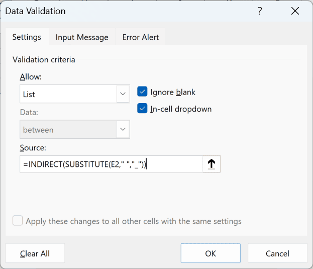
If column E is still empty, Excel warns that the Source currently evaluates to an error. Click Yes, as the list works once a category is picked.
Now, when you make a selection in the Category drop-down, the options in the dependent drop-down automatically update.
How does this work?
When you select Furniture in E2, the INDIRECT function turns that text into a reference to the named range Furniture, so the drop-down lists all the furniture items.
The reason for the SUBSTITUTE function is that Excel does not allow spaces in named ranges.
So when you create a named range from a two-word heading like Office Supplies, Excel names it Office_Supplies.
The SUBSTITUTE function converts the space in E2 into an underscore, so the INDIRECT function finds the right name.
If none of your categories have a space in them, the simpler formula =INDIRECT(E2) works as well.
Note that the named ranges cover rows 2 to 6 for every category, so shorter lists (such as Office Supplies) show a blank option at the end of the drop-down.
Also, if you rename a category heading later, you need to create the names again.
Follow along with the example file
Dependent Drop Down List in Excel.xlsx
Highlight Wrong Selections in the Dependent Drop Down
There is one problem with all the methods above.
When you change the first drop-down after making a selection in the dependent drop-down, the dependent drop-down does not change.
For example, if you select Furniture as the category and Chairs as the sub-category, and then go back and change the category to Electronics, the sub-category still shows Chairs.
A simple conditional formatting rule can highlight the cell whenever there is a mismatch, so you can see it and correct it.
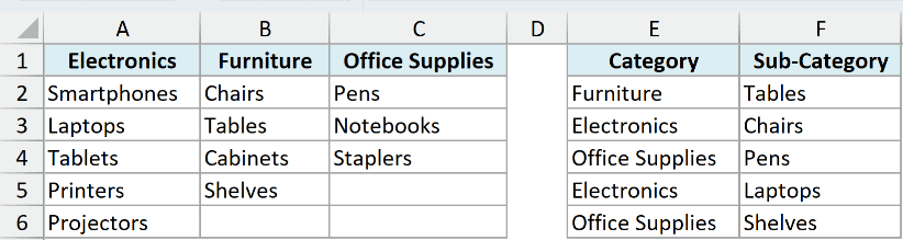
Below I have Category and Sub-Category drop-downs in columns E and F, and I want to highlight sub-categories that don’t match the selected category.
Rows 3 and 6 have a sub-category that doesn’t belong to the category.
Here are the steps to highlight mismatches in the dependent drop-down list:
- Select the cells that have the dependent drop-down list (F2:F6 in this example).
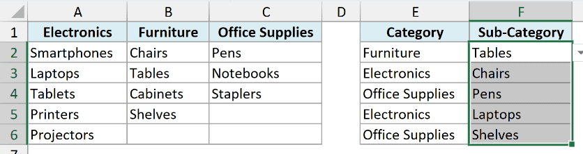
- Go to Home, then Conditional Formatting, then New Rule.
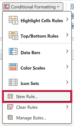
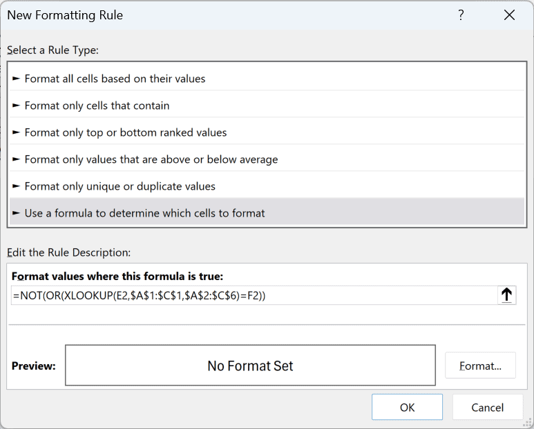
- In the New Formatting Rule dialog box, select ‘Use a formula to determine which cells to format’.
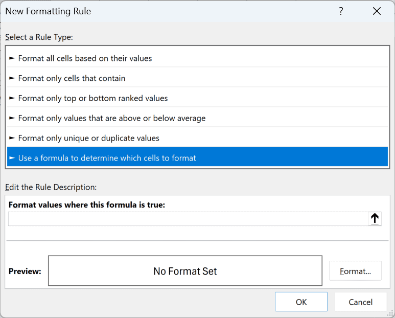
- In the formula field, enter the formula below.
=NOT(OR(XLOOKUP(E2,$A$1:$C$1,$A$2:$C$6)=F2))
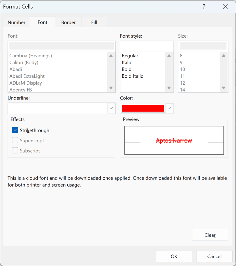
- Click the Format button, and in the Font tab, check Strikethrough and set the Color to red.
- Click OK, and then click OK again.
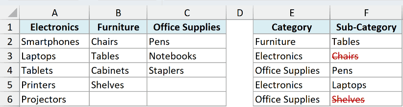
Now Chairs (under Electronics) and Shelves (under Office Supplies) show in red with a strikethrough. As soon as you pick a valid sub-category, the formatting goes away.
How this formula works:
- XLOOKUP(E2,$A$1:$C$1,$A$2:$C$6) – This returns all the items for the category selected in E2.
- …=F2 – This compares each of those items with the value in F2 and gives a TRUE for a match and FALSE otherwise.
- OR(…) – This returns TRUE if any one of them matched, which means the selection is valid.
- NOT(…) – This flips the result, so a mismatch returns TRUE, and that tells conditional formatting to format the cell.
Note that this rule highlights the wrong selection but does not change it. The old value stays in the cell until you pick a new one.
Also, since this rule uses XLOOKUP, it needs Excel 2021 or later. If you’re on Excel 2019 or earlier, use this formula in the same rule instead:
=ISERROR(VLOOKUP(F2,INDEX($A$2:$C$6,,MATCH(E2,$A$1:$C$1,0)),1,0))
The MATCH function finds the column of the selected category, and the INDEX function returns that column of items.
The VLOOKUP function then looks for F2 in those items.
If F2 isn’t in that column, the VLOOKUP function returns an error. The ISERROR function turns that error into TRUE, so conditional formatting highlights the cell.
You can see this rule on the INDIRECT Method sheet in the example file.
Show “Please Select” Instead of the Wrong Selection
Instead of highlighting a wrong selection, you can make it disappear and show a message such as Please select in its place.
This uses the same formula, with a custom number format instead of a strikethrough.
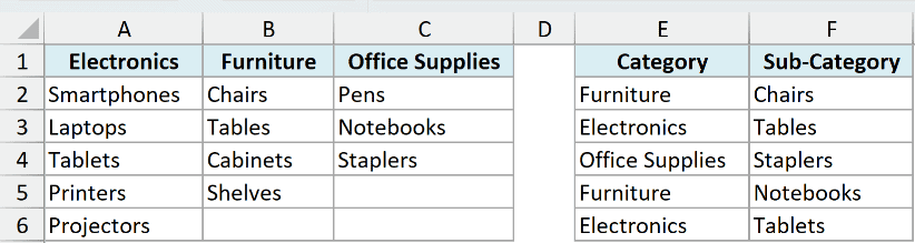
Below I have Category and Sub-Category drop-downs in columns E and F, and I want column F to show Please select when the selections don’t match.
Rows 3 and 5 have a sub-category that doesn’t belong to the category.
Here are the steps:
- Select F2:F6, go to Home, then Conditional Formatting, then New Rule.
- Select ‘Use a formula to determine which cells to format’, and enter =NOT(OR(XLOOKUP(E2,$A$1:$C$1,$A$2:$C$6)=F2)) in the formula field.
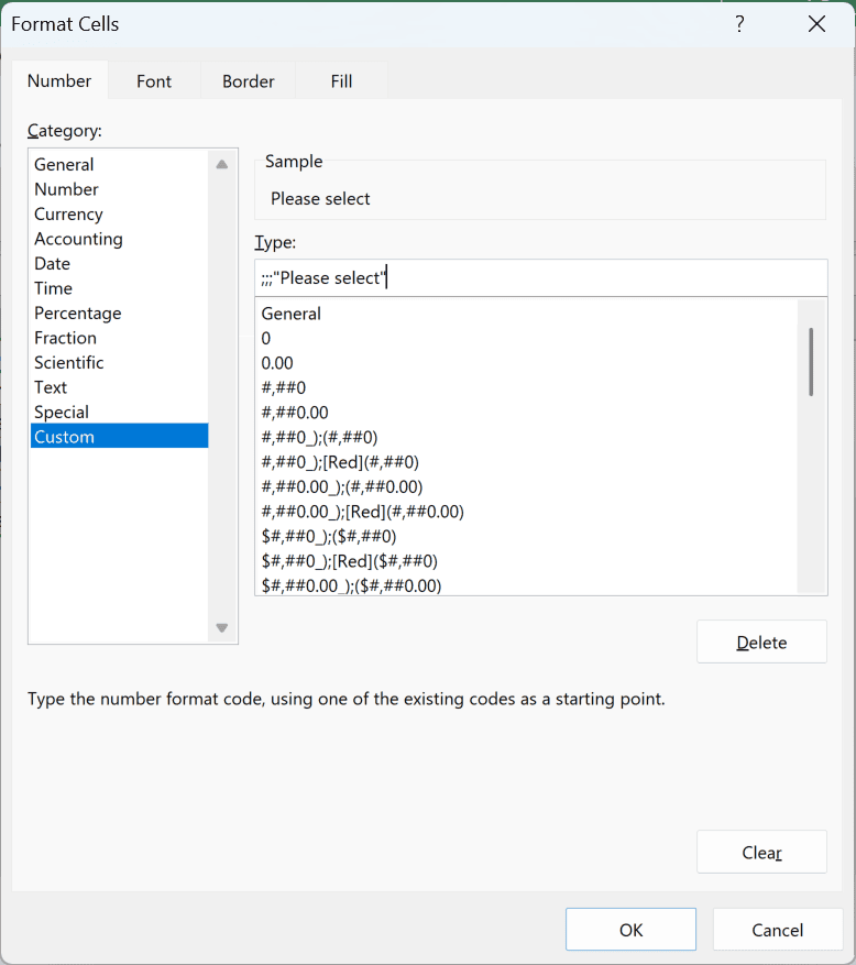
- Click Format, and in the Number tab, select Custom and enter ;;;”Please select” in the Type field.
- Go to the Font tab, set the Color to red, and click OK twice.
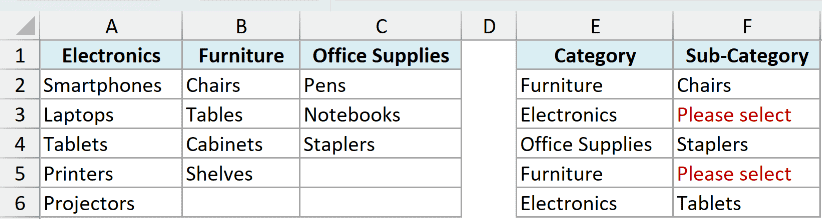
Now F3 and F5 show Please select in red, and they go back to normal as soon as you pick a valid sub-category.
A custom number format has four parts separated by semicolons: positive numbers, negative numbers, zeros, and text.
By leaving the first three empty and putting “Please select” in the text part, any text in the cell displays as Please select.
Important: The wrong value is still in the cell. You can see it in the formula bar, and any formula that refers to this cell still uses it.
Clear the Dependent Drop Down Automatically Using VBA
If you want the dependent drop-down to actually reset whenever the main drop-down changes, you need VBA.
I personally prefer the conditional formatting method, because VBA code needs a macro-enabled file, and the person you share it with has to enable macros.
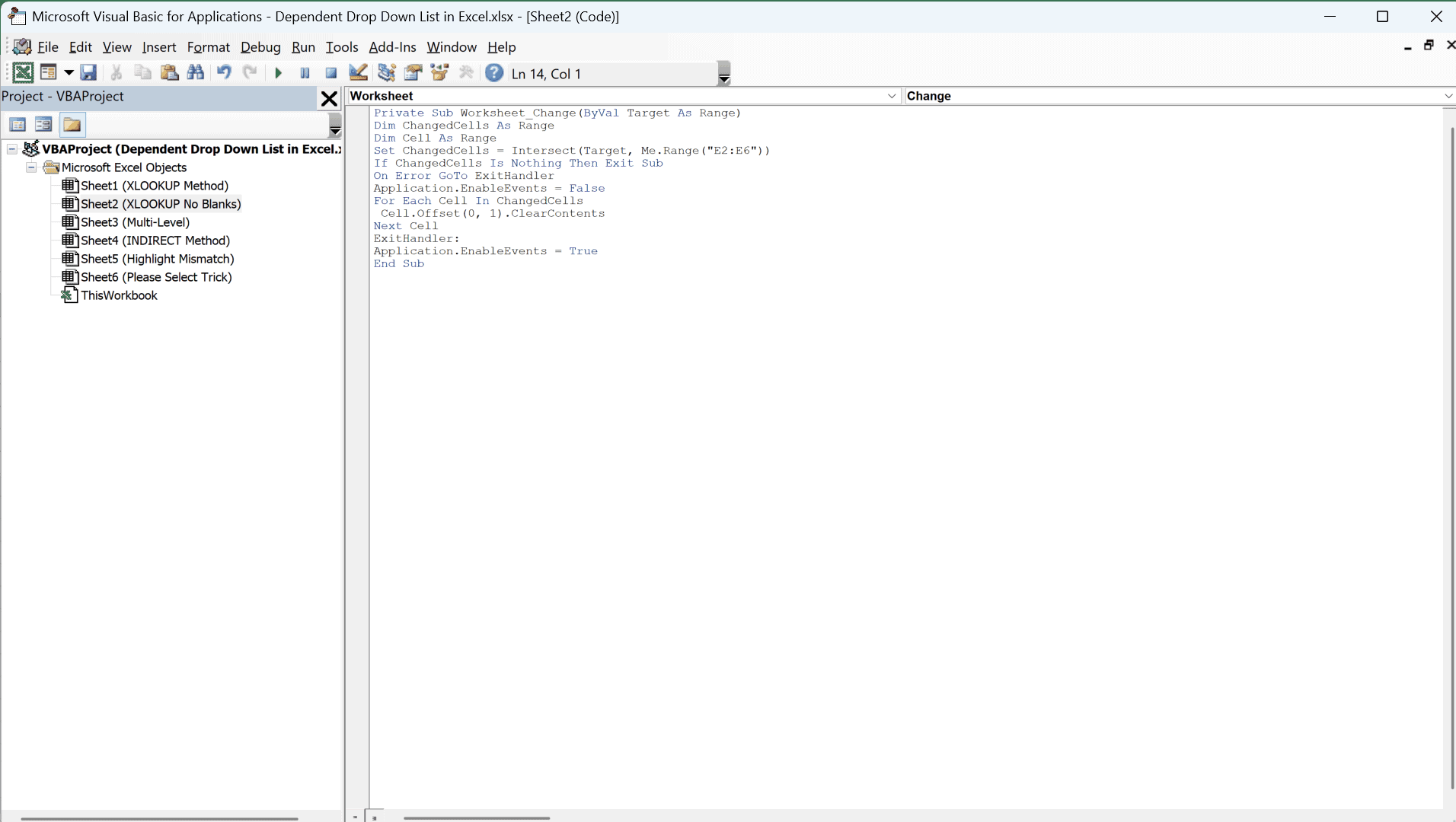
Here is the VBA code to clear the contents of a dependent drop-down list:
Private Sub Worksheet_Change(ByVal Target As Range)
Dim ChangedCells As Range
Dim Cell As Range
Set ChangedCells = Intersect(Target, Me.Range("E2:E6"))
If ChangedCells Is Nothing Then Exit Sub
On Error GoTo ExitHandler
Application.EnableEvents = False
For Each Cell In ChangedCells
 Cell.Offset(0, 1).ClearContents
Next Cell
ExitHandler:
Application.EnableEvents = True
End SubThis code uses the Worksheet_Change event, so it runs whenever a cell changes on the sheet.
If the changed cells are in E2:E6 (where the Category drop-downs are), it clears the cell to the right of each one (the dependent drop-down). Changes anywhere else on the sheet are ignored.
If your main drop-downs are in a different range, change E2:E6 in the code to that range.
This code is based on this tutorial by Debra on clearing dependent drop down lists in Excel when the selection is changed.
Here is how to make this code work:
- Copy the VBA code.
- In the workbook that has the dependent drop-down list, go to the Developer tab, and in the Code group, click on Visual Basic (or use the keyboard shortcut ALT + F11).

- In the Project Explorer on the left, you’ll see all the worksheet names. Double-click on the sheet that has the drop-down list.
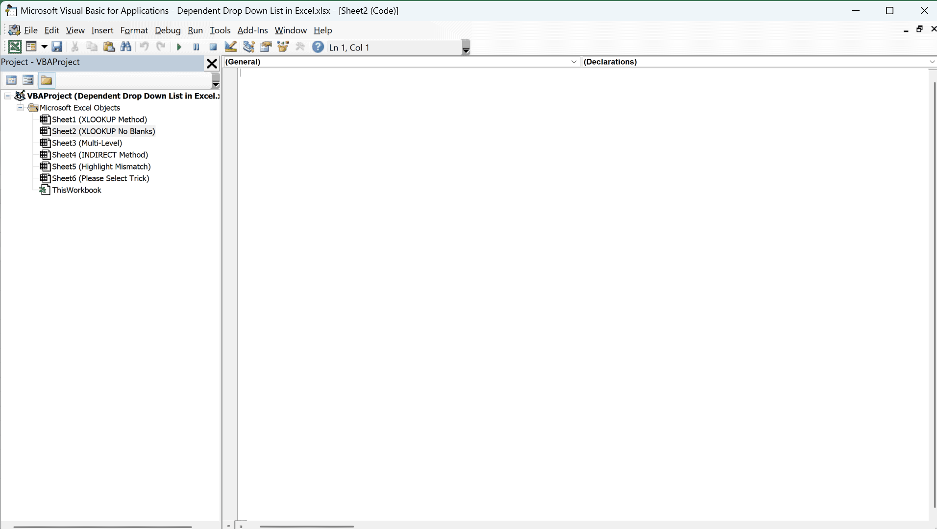
- Paste the code in the code window on the right.
- Close the VB Editor.
Now, whenever you change the main drop-down, the code clears the dependent drop-down next to it.
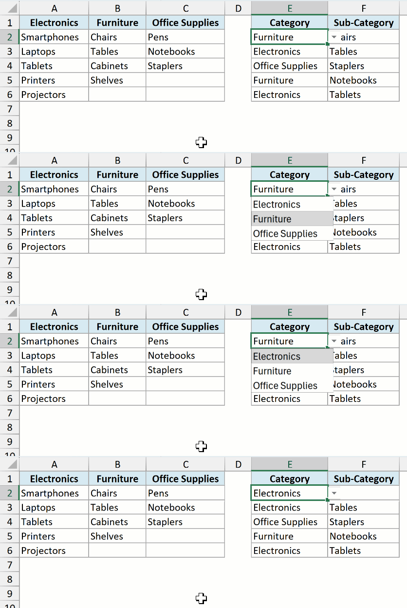
If you’d rather show a message than an empty cell, replace the ClearContents line with Cell.Offset(0, 1).Value = “— Make Selection —“.
Important: Save the file as a macro-enabled workbook (.xlsm). If you save it as a regular .xlsx file, the code is removed.
Also note that you can’t undo a change made by VBA, so the cleared value can’t be brought back with Control + Z.
So these are the ways you can create a dependent drop-down list in Excel, along with a few ways to handle wrong selections when the first drop-down changes.
I hope you found this Excel tutorial useful.
Other Excel Articles You May Also Like:
- Extract Data based on a drop-down list selection
- Creating a drop-down list with search suggestions
- Select multiple items from a drop-down list
- Create multiple drop-down lists without repetition
- Save Time with Data Entry Forms in Excel
- Create Data Validation List from Excel Table as Source
- Display Main and Subcategory in Drop Down List in Excel
- How to Make a Yes/No Drop-Down in Excel
- Enable Conditional Data Entry in Excel using Data Validation

Doesn’t work. Says “The Source currently evaluates to an error.” anybody with a simpler way of doing this that actually works and doesn’t require someone to know VBA code?
Small formula correction for those looking to use a conditional color change as opposed to a VBA script to highlight mismatches.
The original formula: =ISERROR(VLOOKUP(E3,INDEX($A$2:$B$6,,MATCH(D3,$A$1:$B$1)),1,0))
Needs to have a “0” (zero) added to the MATCH function’s third argument. The updated formula is:
=ISERROR(VLOOKUP(E3,INDEX($A$2:$B$6,,MATCH(D3,$A$1:$B$1,0)),1,0))
For MATCH, zero is an implied default, but some of you – like me – may have had formatting issues based on the original formula due to how it processes the range. This error – for me – was being caused by the MATCH function… so forcing a “0” in the third argument makes for an exact match. Otherwise, you have to sort your menu and that’s a pain.
To the author… excellent post and thank you!
I want to use 3 or more drop down lists but is showing error
Please help
Two teammates and I have been unsuccessful in building a spreadsheet with one drop down list and two dependent drop down lists. We can create a drop down list of five “entities” in column one. We can create a dependent drop down list of “expense categories” in column two which only shows the relevant “expense categories” of the “entity” selected in column one. We can not figure out how to create a second dependent drop down list of “expense details” in column three which only shows the relevant “expense details” of the “expense category” selected in column two. Any help would be greatly apreciated! I would be willing to pay for assistance or make a donation to the favorite charity of anyone who could help.
This method seem not to be working anymore with the latest version of Excel and Windows. I am running version Office 365 MSO (16.0.12325.20328) on Windows 10 Pro version 1909.
This is extremely frustrating. I have been using this type of lists for years using indirect to “construct” range names, where the range name reference the list to be used.
Can someone please tell me why indirect lost the functionality to construct name ranges in data validation to create lists?
Hello Theron.. I am on Office 365 ProPlus and this method is working for me. I am using Version 1908. It’s possible that there could be an issue with a specific version. I have not heard anything about it but will search and see if I can find anything
Thank you Sumit,
If not for your comment I would not have done the above to the letter. It works now.
I can say why it did not worked initially. My name range was defined in the “Refer to:” section as =OFFSET(CatPr,0,0,COUNTA(Data!$L:$L)-2,1). This was to ensure we can add more items and not showing blank spaces. However, it seems that indirect does not like it when the name range has a formula in the “Refer to:” section. Which is silly, is it not?
Regardless, Thanks
Thank you so much for the clear instructive and useful information
What if we have a additional column of “Groceries” with “Vegetable” and “Fruit” ?..i am getting values of main column as Fru./Vege./Groc.. but in dependent column i am not getting values …what i am doing wrong ?
I have a 3 dependant drop down list (N dependant on M, M dependant on L). and for some reason my code below seem to work as such, hope it helps:
On Error Resume Next
If Target.Column = “$L” Then
If Target.Validation.Type = “$M” Then
Application.EnableEvents = False
Target.Offset(0, 1).ClearContents
just realised that for some reason it affects other column not defined by my above codes. any idea how I can prevent that?
hi
First of all, this is one of the best tutorial! Thanks.
I had a problem with your guidance. when I used your formula ” =INDIRECT(SUBSTITUTE(E5,” “,”_”)) ” Excel show me this error: (a named range you specified cannot be found)
Please change ” (E3,” “,”_”) ” to (E5,” ”,”_”).
Maybe someone like me is enough lazy to just copy the formula!!!
Thank you very much.
Works great, although when I open the dependent dropdown, it defaults to the last item on the list. Any way to make it default to the top?
shit
I have everything working correctly for the second drop down, until I get to the end and I hit OK then it tells me “the Source currently evaluates to an error. Do you want to continue?
Could this be because my first drop down has numbers? I don’t know why else it would not work ?! any help would be great!
Hi Danielle, it is due to the fact this this method is not supported anymore. I would like someone to comment why the use of the indirect function is not working anymore.
fff
The VBA code only works in your sample worksheet, if i shift the dropdown columns to the right and change the vba code accordingly it does not work. How can i get hte code to work?
I had a similar problem in that my drop down menus were in columns F and G rather than D and E. To get the VBA code to work, I changed the line “If Target.Column = 4 Then” to “If Target.Column = 6 Then”, since F is the sixth column. The second drop down menu would then clear. Hope this helps someone.
I want to use the VBA code, but I would need to add it to code already existing for the worksheet. How would you make this work?
Any thoughts how to select both fruits and vegies as multi select ( in A) followed by list of fruits and vegies in column B
Been looking for this as well. Any luck?
How about if fruits and vegetables have different number of items? Let’s say fruits has 5 items and vegetables has 3 items, if vegetables is selected then in drop down 2 has 2 blank items. Is there a way to eliminate those 2 blanks in drop down 2?
Use ctrl-select only the cells you wish to use. This allows you to omit any blank cells during the “Formulas -> Create from Selection” step.
I tried that. But it created an error: “This selection isn’t valid. Make sure the copy and paste areas don’t overlap unless they are the same size and shape.”
Any ideas, or sample file?
Owh, never mind. Solved it by defining name for each selection. Thanks.
If i need to create named range (dependent) for cars depending on the brand but they don´t have a fixed number of cars. Does this mean I have to define the range manually per brand instead of “create for selection”? is there any way we could use remove the blank spaces automatically?
I’m getting an error “A named range ou specified cannot be found.”
How can i link this drop down to dashboard or chart? please help me
Very useful tutorial. Thanks
Thank you. It was pretty clear and useful.
Excellent content, thank you for your expertise and help!
Thanks mate – very helpful
Thank you sooo much.. very useful
Very Nicely explained and very useful. Thanks
Mine isn’t working. I followed the steps exactly, but my second row for lists shows an arrow for a dropdown list, but doesn’t actually create a dropdown list based on the choice made in the first column.
For clarification, when I attempt the second part of the Data Validation, I get an error message saying “The Source currently evaluates to an error.” But the first selection works just fine. Can someone please help me?
Hey Kyle this happen to me as well. You cannot have spaces anywhere you are making a drop down list. Your list may have been two words like yellow car. Instead you would have to put yellow_car. Put underscores for all of your spaces and it should work
Yeah, that wasn’t it. I was running only one word options, but I forget that this message happens, but wasn’t related to the multi-multi-tiered hierarchy. I still can’t do a three+ level hierarchy of dropdowns.
I am having the same issue. I cant get the 2nd selection to create the drop down. any ideas?
for this formula —- what if I had three columns in my named ranged (not two) how would the match formula change?
formula: =ISERROR(VLOOKUP(E3,INDEX($A$2:$B$6,,MATCH(D3,$A$1:$B$1)),1,0))
I have the same question!
you’re the best, thank you so much
it was the good one
I had one excel file with complete functions and formulas along with logic and examples. Unfortunately, I had missed that file. If you have these kind of file, please share the same with me. Thanks…
hi, i have the same trouble as Abhishek Goyanka,
was this solved?
Creating a Dependent Drop Down List in Excel
I have categories name with White spaces, drop down is not working in that case.
Any solution
Excellent stuff
Thanks
good
Very excellent job, thank you very much.
Very Helpfull task
Wow! This was so helpful and exactly what I was looking for. I knew the solution had to be much more simple than I was originally planning to try.
Hi Could you possibly help me with a slightly bigger formula?
Where did my comment go?
I have a issue with name box in excel, which does not accept hypen “/” for eg: “AM/NAME” , please give me suggestion for this issue.
i am trying to populate dependent drop down box
HI, How can I make the drop down list works for multiple cells and not just in a unique cell?
thanks alot very usefull trick
Hi Sumit,
How to update the dependent list when you change primary list after initially making some selection? Right now if you select the US and then Alaska, after that if you change it to India, the state still remains Alaska. Please help.
Thanks
Hello Abhishek.. This can be done using VBA. Will try and create it and share with you
Hi Sumit,
Really appreciate the help. Please let me know if you are able to write VBA script which accomplishes the task. Thanks again.
I want to create two cells dependent on the data entered into the first cell. So say I have a list of Company Branches listed by city. Then I have 6 multiple lists that list the Foremen that work in each city AND I have 6 lists of Superintendents that work in each city. I created the city list in cell B2. In the Superintendents cell E3 I used =Indirect(B2) and it lists all the Superintendents working in the city showing. Now in cell E2 I want to have the Foremen that work in each city. I tried =Indirect(B2) which gives me the same list in cell E3. How do I get E2 tied to B2????
i have my drop down all done, but when i to look at the list , there is nothing showing, can you help me please
Hi there, is there any way you know to do this but with a list of all countries and regions of the world without having to create as many columns as countries exist? I have the list with two columns, each row per region/country… When I select one of the countries, I need the drop down list to display all the regions of that country.
Thanks Sumit for sharing this! However, I have find two errros:
1 – While addition to the data set (As states) and consequently using indirect formula as Indirect(States Name) doesn’t show any options in list.
2 – Is there any way in which cells should appear empty for that particular row if we change any data set?
Hey Sumit, I have a doubt – when you choose US in Cell -E2 then the other drop down list in cell:F2 shows US cities. Lets assume, we select Alaska as city in F2 but at the same time we change the country again US to India in E2, then F2 field still shows Alaska.
Is there a way cell should appear empty if we change the country ?
How do i fix this? its not letting me do the data validation following the exact steps.
I also have the same mistake…anybody could fix it?
Thanks!!!
How would you this with a third drop down based on BOTH the previous drop downs? For instance, adding a “City.”
Hi Tyler.. Thanks for dropping in.. You can create the third drop down in the similar way. In this case. city would be dependent on selected state. You would need to create named ranges for all states, and the formula would be =INDIRECT(States Name)