How to Flip Data in Excel (Reverse Order of Rows or Columns)

If you want to flip data in Excel, there are a few ways to do it.

By that I mean reversing the order of the data upside down in a vertical dataset or left to right in a horizontal dataset.

Now, if you’re thinking that there must be an inbuilt feature to do this in Excel, I’m afraid you’d be disappointed.

There’s no Reverse button on the worksheet itself (Power Query has one, which I cover below).

But you can easily do this using a simple sorting trick, formulas, Power Query, or VBA.

In this tutorial, I will show you how to flip the data in rows, columns, and tables in Excel.

I’ll start with flipping data vertically (reversing the rows), and then show you how to flip it horizontally (reversing the columns).

So let’s get started!

Flip Data Vertically (Reverse Rows Upside Down)

Let’s start with the more common case, where your data is in a column (or a table) and you want the last row to come first.

Flip Data Upside Down Using Sort and a Helper Column

One of the easiest ways to reverse the order of the data in Excel would be to use a helper column and then use that helper column to sort the data.

Note that simply sorting the names Z to A won’t do it. That sorts them alphabetically, which isn’t the same as reversing them.

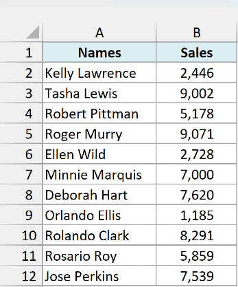
Suppose you have a data set of names and their sales as shown below and you want to flip this data:

Below are the steps to flip the data vertically:

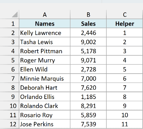
1. In the adjacent column, enter ‘Helper’ as the heading for the column (cell C1 here)

2. In the helper column, enter a series of numbers (1, 2, 3, and so on). You can use the methods shown here to do this quickly

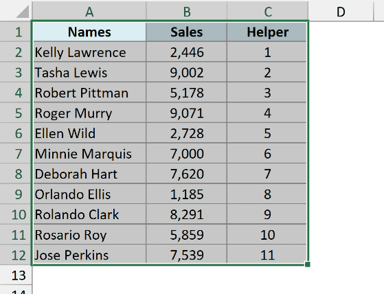
3. Select the entire data set including the helper column (A1:C12)

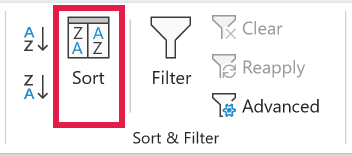
4. Click the Data tab and then click on the Sort icon

5. In the Sort dialog box, select ‘Helper’ in the ‘Sort by’ drop-down (make sure ‘My data has headers’ is checked)

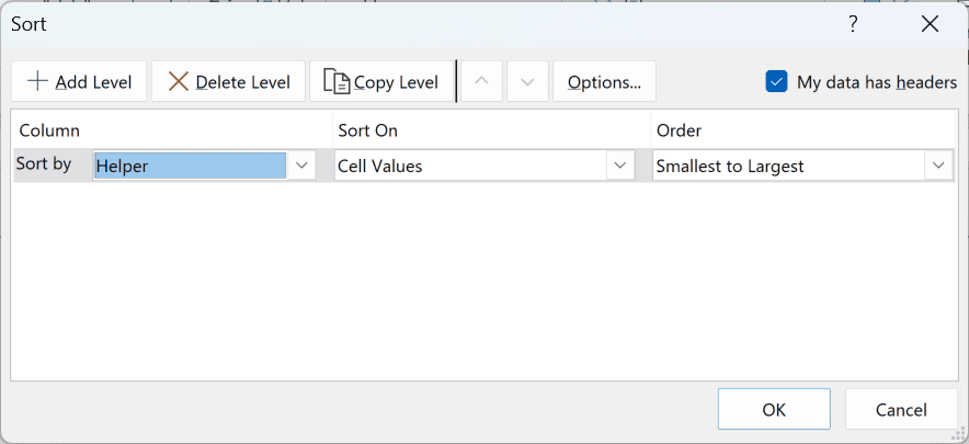
6. In the Order drop-down, select ‘Largest to Smallest’

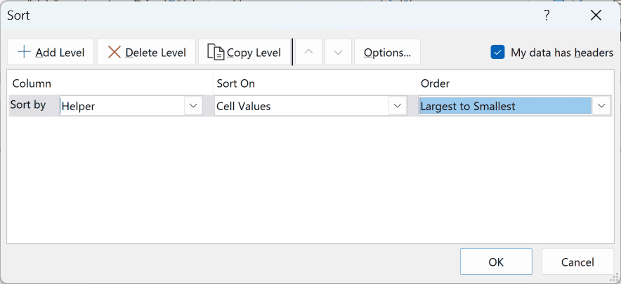
7. Click OK

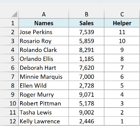
The above steps would sort the data based on the helper column values, which would also lead to reversing the order of the names in the data.

Once done, feel free to delete the helper column.

If you might need the original order back later, keep the helper column. Sorting it Smallest to Largest will undo the sort.

Pro Tip: Once the helper column is in place, you can skip the dialog box. Select any cell in the helper column and click the Z→A sort button in the Data tab.

In this example, I’ve shown you how to flip the data when you just have a couple of columns, but you can also use the same technique if you have an entire table.

Just make sure that you select the entire table and then use the helper column to sort the data in descending order.

Also read: How to Move Columns in Excel

Reverse Order Using the SORTBY Formula

Excel 2021, Excel 2024, and Microsoft 365 have some new formulas that make it really easy to reverse the order of a column or a table in Excel.

In this section, I’ll show you how to do this using the SORTBY formula. If you’re on Excel 2019 or older, use the INDEX formula method shown further down.

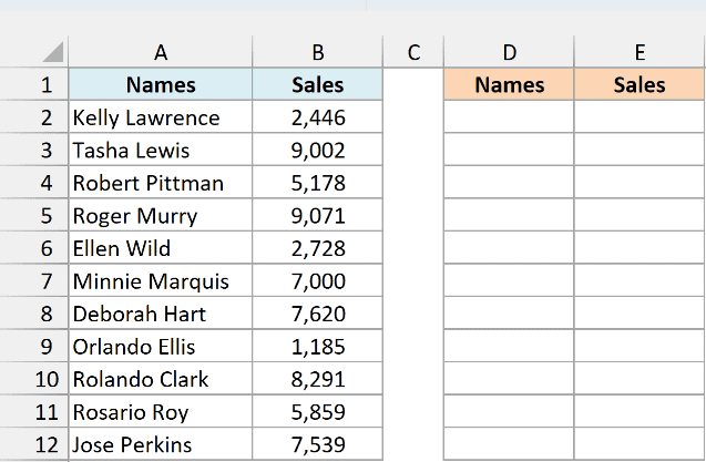
Suppose you have a table as shown below and you want to flip the data in this table:

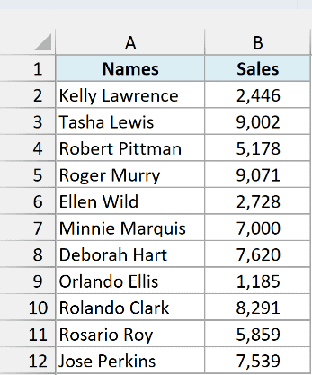
To do this, first, copy the headers and place them where you would want the flipped table (D1:E1 here).

Now, use the following formula in cell D2, right below the left-most header:

=SORTBY(A2:B12,ROW(A2:A12),-1)

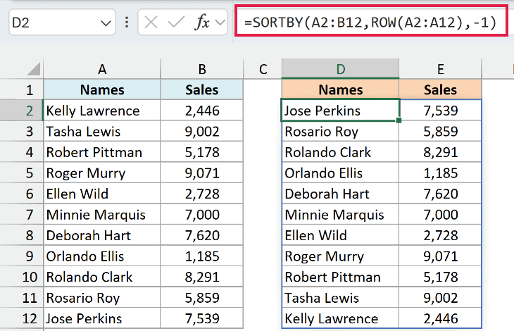
This one formula spills down and fills the entire reversed table in D2:E12. You don’t need to copy it down.

The above formula sorts the data by using the result of the ROW function as the basis to sort it.

The ROW function in this case would return an array of numbers that represents the row numbers in the specified range (which in this example would be 2, 3, 4, and so on up to 12).

And since the third argument of this formula is -1, it would force the formula to sort the data in descending order.

The record that has the highest row number would come at the top and the one which has the lowest row number would go at the bottom, essentially reversing the order of the data.

If anything is in the cells where the result will go, you’ll get a #SPILL! error instead of the result. Make sure those cells are empty before entering the formula.

Once done, you can convert the formula to values to get a static table.

Note: When you use a formula to reverse the order of a data set in Excel (this applies to every formula in this article), it would not retain the original formatting.

If you need the original formatting on the sorted data as well, you can apply it manually.

Or you can copy and paste the formatting from the original data set to the new sorted dataset.

If you’re using Microsoft 365 or Excel 2024, here’s an even shorter formula that does the same thing:

=CHOOSEROWS(A2:B12,-SEQUENCE(ROWS(A2:B12)))

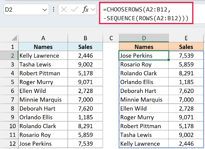
How this formula works:

• ROWS(A2:B12) counts the rows in the data, which is 11.
• The SEQUENCE function then gives the numbers 1 to 11, and the minus sign in front turns them into -1 to -11.
• CHOOSEROWS treats a negative number as a position counted from the bottom. So -1 is the last row, -2 is the second-last row, and so on.

Also read: How to Swap Cells in Excel?

Reverse Order Using INDEX (Excel 2019 and Older)

In case you don’t have access to the SORTBY function, worry not – you can use the amazing INDEX function.

Suppose you have a dataset of names as shown below and you want to flip this data.

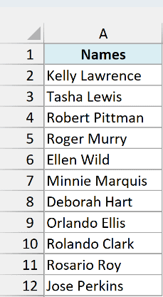
Below is the formula to do this (enter it in cell C2 and copy it down to C12):

=INDEX($A$2:$A$12,ROWS(A2:$A$12))

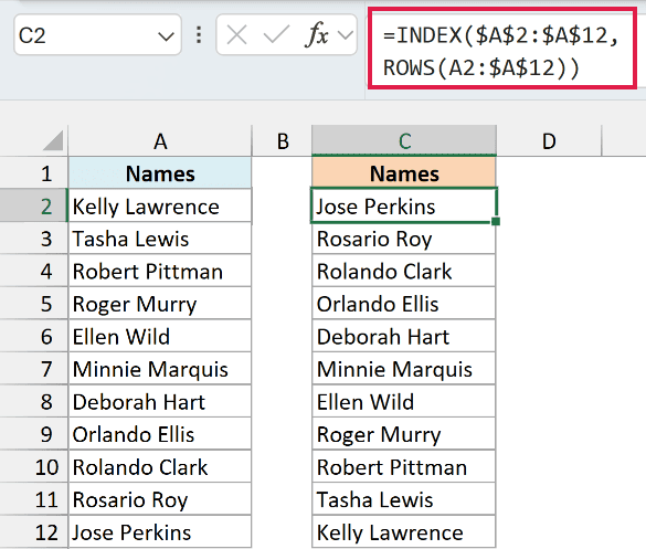
How does this formula work?

The above formula uses the INDEX function that would return the value from the cell based on the number specified in the second argument.

The real magic happens in the second argument where I have used the ROWS function.

Since I have locked the second part of the reference in the ROWS function, in the first cell, it would return the number of rows between A2 and A12, which would be 11.

But when it goes down the rows, the first reference would change to A3, and then A4, and so on.

The second reference would remain as is because I have locked it and made it absolute.

As we go down the rows, the result of the ROWS function would decrease by 1, from 11 to 10 to 9, and so on.

And since the INDEX function returns us the value based on the number in the second argument, this would ultimately give us the data in the reverse order.

Unlike the SORTBY function, this formula doesn’t spill. That’s why you need to copy it down for every row.

You can use the same formula even if you have multiple columns in the data set.

However, you will have to add a third argument that would specify the column number from which the data needs to be fetched.

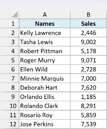
Suppose you have a data set as shown below and you want to reverse the order of the entire table:

Below is the formula that will do that for you (enter it in cell D2, then copy it down and to the right):

=INDEX($A$2:$B$12,ROWS($A2:$A$12),COLUMNS($A$2:A2))

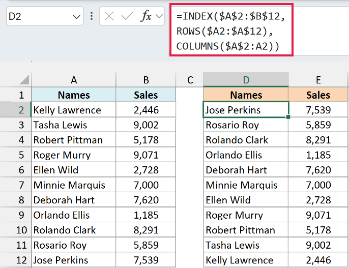
This is a similar formula where I’ve also added a third argument that specifies the column number from which the value should be fetched.

To make this formula dynamic, I have used the COLUMNS function that would keep on changing the column value from 1 to 2 to 3 as you copy it to the right.

I’ve also put a dollar sign before the A in $A2. This keeps the ROWS function pointing at column A when you copy the formula to the right.

Once done, you can convert the formulas to values to make sure that you have a static result.

Reverse Rows Using Power Query

If you want a one-click option, Power Query has a Reverse Rows command. It also helps when your list keeps growing, since you can refresh the result instead of redoing the flip.

Power Query is available in Excel 2016 and later versions, including Microsoft 365, as Get & Transform in the Data tab.

Below I have the same names and sales data, which I have converted into an Excel Table.

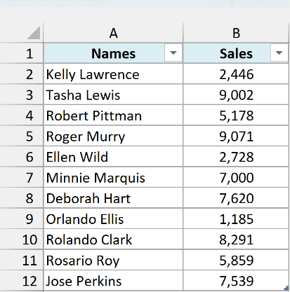
Here are the steps to reverse the rows using Power Query:

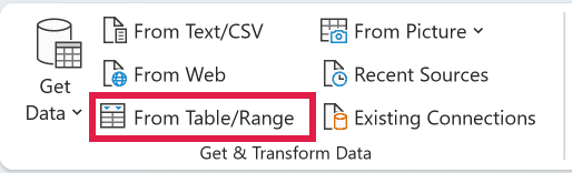
1. Select any cell in the data, click the Data tab, and then click on From Table/Range (if your data isn’t a table yet, Excel asks you to create one, so click OK)

2. In the Power Query Editor, click the Transform tab and then click on Reverse Rows

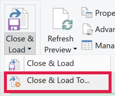
3. Click the Home tab, click the Close & Load drop-down, and then click on Close & Load To

4. In the Import Data dialog box, select Table and Existing worksheet, enter =$D$1 as the location, and click OK

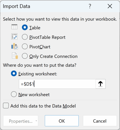
The reversed data now loads into D1:E12 as a new table.

Depending on your Power Query settings, you may also see a Changed Type step in the Applied Steps pane, right before Reversed Rows. That’s fine, leave it as is.

When you add new rows to the source table, right-click the result and click Refresh (or use Refresh All in the Data tab), and Power Query flips the updated list again.

Flip Data Using VBA

If flipping the data in Excel is something you have to do quite often, you can also try the VBA method.

With a VBA macro code, you can copy and paste it once within the workbook in the VBA editor, and then reuse it over and over again in the same workbook.

You can also save the code in the Personal Macro Workbook or as an Excel add-in and be able to use it in any workbook on your system.

Below is the VBA code that would flip the selected data vertically in the worksheet.

Sub FlipVertically()

'Code by Sumit Bansal from trumpexcel.com

Dim TopRow As Variant
Dim LastRow As Variant
Dim StartNum As Long
Dim EndNum As Long

Application.ScreenUpdating = False

StartNum = 1
EndNum = Selection.Rows.Count

Do While StartNum < EndNum
TopRow = Selection.Rows(StartNum)
LastRow = Selection.Rows(EndNum)
Selection.Rows(EndNum) = TopRow
Selection.Rows(StartNum) = LastRow
StartNum = StartNum + 1
EndNum = EndNum - 1
Loop

Application.ScreenUpdating = True
End Sub

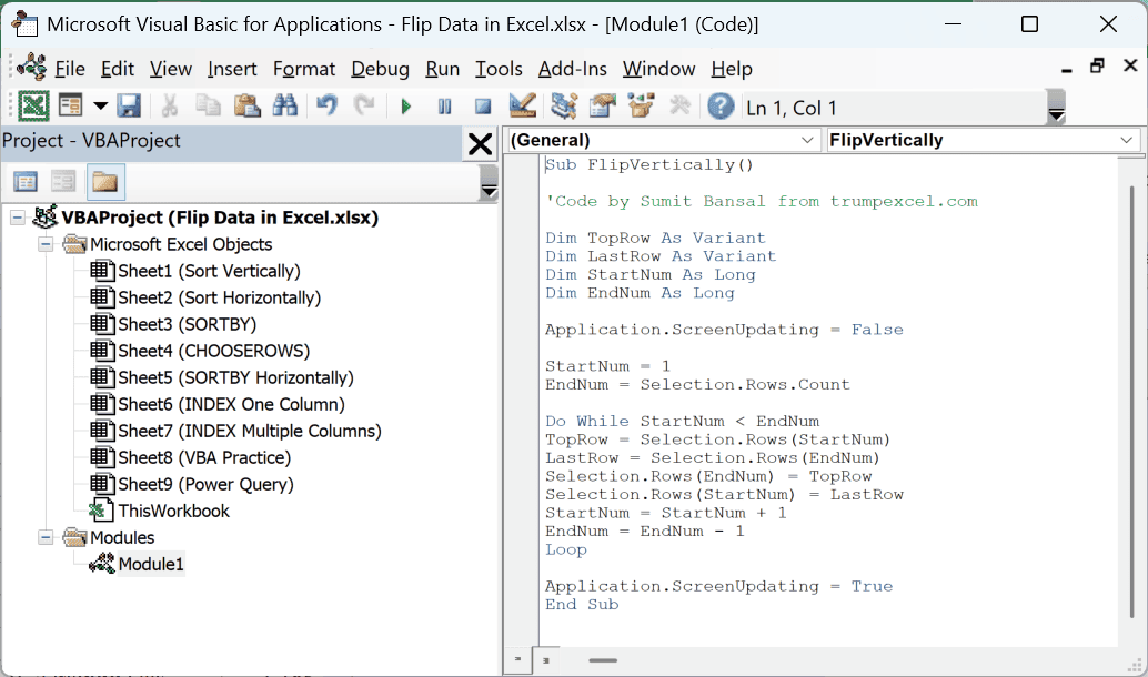
Sub FlipVertically()'Code by Sumit Bansal from trumpexcel.comDim TopRow As VariantDim LastRow As VariantDim StartNum As LongDim EndNum As LongApplication.ScreenUpdating = FalseStartNum = 1EndNum = Selection.Rows.CountDo While StartNum < EndNumTopRow = Selection.Rows(StartNum)LastRow = Selection.Rows(EndNum)Selection.Rows(EndNum) = TopRowSelection.Rows(StartNum) = LastRowStartNum = StartNum + 1EndNum = EndNum - 1LoopApplication.ScreenUpdating = TrueEnd Sub

To use this code, you first need to make the selection of the data set that you want to reverse (excluding the headers), and then run this code.

Important: A macro can’t be undone with Control + Z. Save a copy of your data before you run it.

How does this code work?

The above code first counts the total number of rows in the data set and assigns that to the variable EndNum.

It then uses the Do While loop where the sorting of the data happens.

The way it sorts this data is by taking the first and the last row and swapping these. It then moves to the 2nd row and the second last row and then swaps these.

Then it moves to the third row and the third last row, and so on. The loop ends when all the sorting is done.

It also uses the Application.ScreenUpdating property and sets it to FALSE while running the code, and then turns it back to TRUE when the code has completed running.

This ensures that you don’t see the changes happening in real-time on your screen, and it also speeds up the process.

Note that the code swaps the values only. Any formulas in the selection become static values, and the cell formatting stays where it was.

How to use the Code?

Follow the below steps to copy and paste this code in the VB Editor (the example file has a VBA Practice tab you can try it on):

1. Open the Excel file where you want to add the VBA code

2. Hold the ALT key and press the F-11 key (you can also go to the Developer tab and click on the Visual Basic icon)

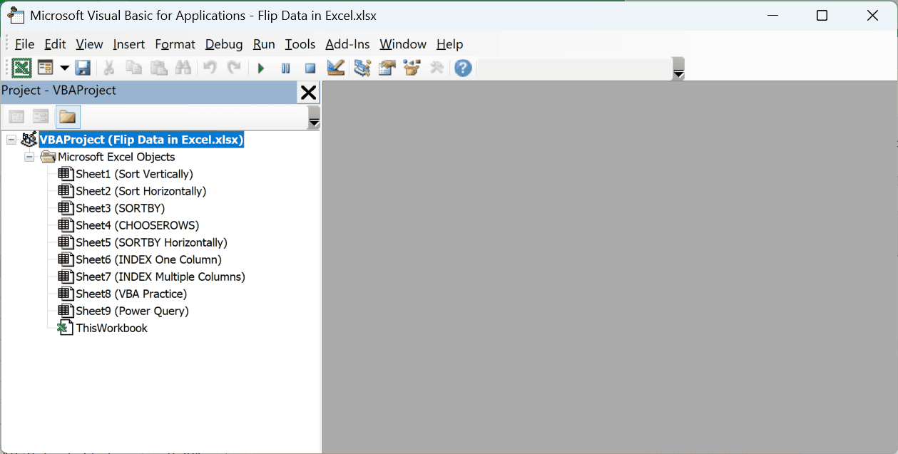
3. In the Visual Basic Editor that opens up, there would be a Project Explorer on the left part of the VBA editor. If you don’t see it, click on the ‘View’ tab and then click on ‘Project Explorer’

4. Right-click on any of the objects for the workbook in which you want to add the code

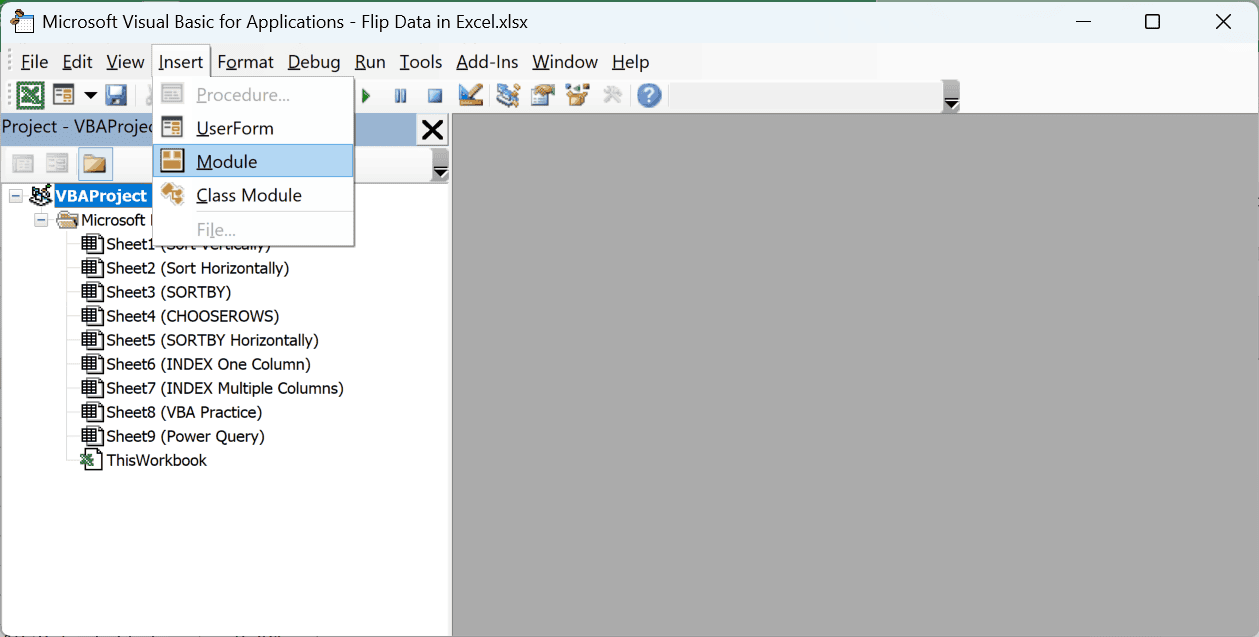
5. Go to the Insert option and then click on Module. This will add a new module to the workbook

6. Double-click on the module icon in the Project Explorer. This will open the code window for that module

7. Copy and paste the above VBA code into the code window

To run the VBA macro code, first select the dataset that you want to flip (excluding the headers).

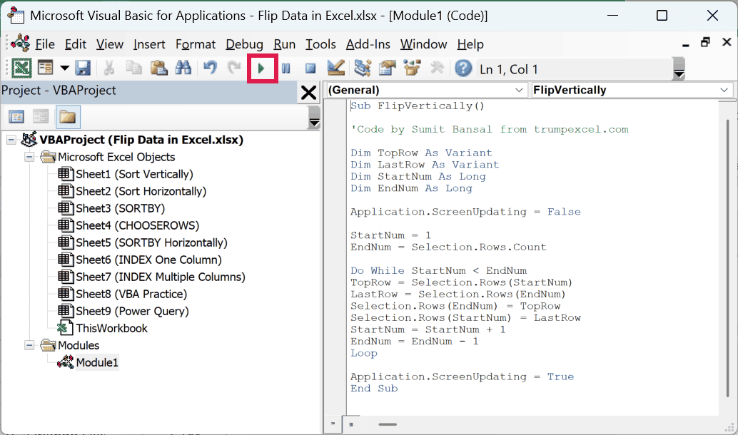
With the data selected, go to the VB Editor and click on the green play button in the toolbar, or select any line in the code and then hit the F5 key.

Since the file now has a macro, save it as a macro-enabled workbook (.xlsm). If you save it as a regular .xlsx file, Excel removes the code.

Flip Data Horizontally (Reverse Columns Left to Right)

Now let’s look at the other case, where your data runs across a row and you want the last column to come first.

Flip a Row Left to Right Using Sort and a Helper Row

You can also follow the same methodology to flip the data horizontally in Excel.

Excel has an option to sort the data horizontally using the Sort dialog box (the ‘Sort left to right’ feature).

Suppose you have a table as shown below, with names in row 1 and sales in row 2, and you want to flip this data horizontally.

Below are the steps to do this:

1. In the row below, enter ‘Helper’ as the heading for the row (cell A3 here)

2. In the helper row, enter a series of numbers (1, 2, 3, and so on)

3. Select the data including the helper row, but leave out the labels in column A (B1:L3 here)

4. Click the Data tab and then click on the Sort icon

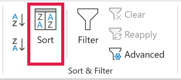
5. In the Sort dialog box, click on the Options button

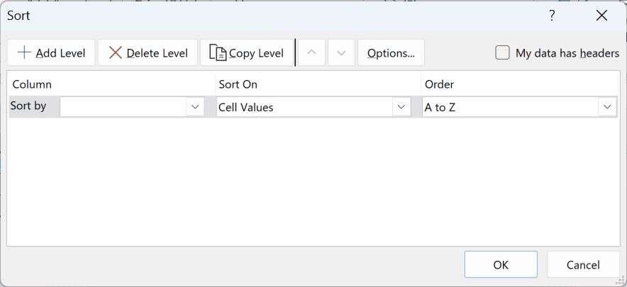
6. In the dialog box that opens, click on ‘Sort left to right’ and then click OK

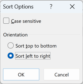
7. In the Sort by drop-down, select Row 3 (or whatever row has your helper numbers)

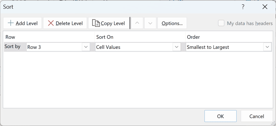
8. In the Order drop-down, select ‘Largest to Smallest’

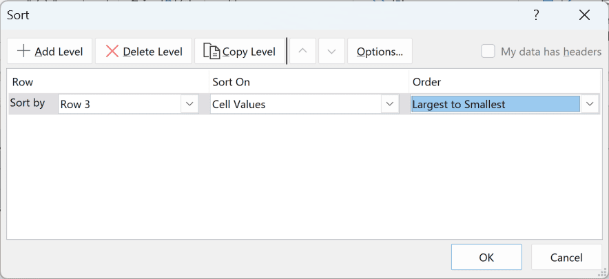
9. Click OK

The above steps would flip the entire table horizontally.

I’ve left column A out because a left-to-right sort has no header option. Excel treats the labels as data, so they can end up at the far right.

Once done, you can remove the helper row.

If what you actually want is to turn rows into columns (and not reverse them), that’s called transposing. Here’s how to transpose data in Excel.

Also read: Convert Columns to Rows in Excel

Reverse Columns Left to Right Using SORTBY

You can use the same SORTBY idea to flip a horizontal dataset, where the last column comes first.

Below I have names and sales arranged horizontally, with the labels in column A, and I want a reversed copy below the original data.

Since the labels in column A shouldn’t move, I’ve copied them to A4:A5 first. Then I’ve used the below formula in cell B4:

=SORTBY(B1:L2,COLUMN(B1:L1),-1)

Like the vertical version, this formula uses position numbers to reverse the data. Here, COLUMN(B1:L1) returns the column numbers 2 to 12.

Those numbers run across a row, so the SORTBY function uses them to sort the columns instead of the rows.

The -1 tells the SORTBY function to sort from largest to smallest, which puts the last column first.

The result spills across B4:L5, so this one formula fills the reversed table.

So these are some of the methods you can use to flip the data in Excel (i.e., reverse the order of the data set).

The sort and SORTBY methods work both vertically and horizontally, as you saw above.

The INDEX, Power Query, and VBA methods are shown for vertical data (you’ll have to adjust the formula and VBA code accordingly for horizontal data flipping).

I hope you found this tutorial useful.

Other Excel tutorials you may also like:

• How to Sort by the Last Name in Excel (Easy Guide)
• How to Sort By Color in Excel (in less than 10 seconds)
• How to Sort Worksheets in Excel using VBA (alphabetically)
• How to do a Multiple Level Data Sorting in Excel
• SORT Function in Excel
• How to Sort Data in Excel using VBA (Range/Columns)

Other Excel Articles You May Also Like:

• TRANSPOSE function