ISNUMBER Function in Excel

The ISNUMBER function in Excel checks whether a cell holds a real number. It returns TRUE if it does and FALSE if it doesn’t, which is handy for catching numbers stored as text.

In this article, I’ll show you how to use ISNUMBER with eight practical examples and explain the results that can catch you out.

Excel ISNUMBER Function Syntax

Here is the syntax of the ISNUMBER function:

=ISNUMBER(value)

• value is the value, cell reference, formula result, or range you want to check. This is the only argument, and it is required.

The ISNUMBER function returns TRUE for numbers, including zero and decimals.

It checks the stored value without converting it. So =ISNUMBER("19") returns FALSE because the double quotes make 19 text.

Other text, blank cells, and logical TRUE/FALSE also return FALSE because none of them is a number.

Give it one cell and you get one answer. Give it a range in Excel 365, Excel 2021, Excel 2024, or Excel for the web, and you get one answer per cell, spilling into nearby cells.

ISNUMBER is available in all Excel versions, including Microsoft 365, Excel 2024, 2021, 2019, and 2016, as well as Excel for Mac and the web.

When to Use the ISNUMBER Function

Use ISNUMBER when you need to:

• Audit imported data for numbers that have arrived as text.
• Check for a number inside IF, data validation, or conditional formatting.
• Turn the positions returned by SEARCH or XMATCH into TRUE/FALSE answers.
• Count or filter entries based on whether they hold a real number.
• Separate numbers from text, blanks, and logical values.

Let me show you a few practical examples of how this works.

Example 1: Check Which Scores Are Real Numbers

Let’s start with a simple example.

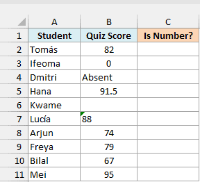
Below is a quiz score sheet, and I want to check which scores are real numbers in column C.

The scores include zero, “Absent”, a blank, and Lucía’s 88 stored as text.

Here is the formula:

=ISNUMBER(B2:B11)

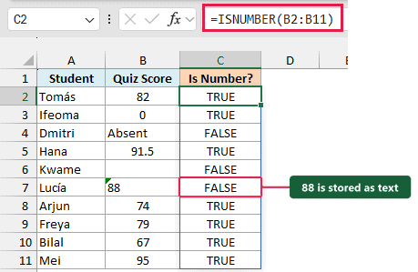
Because you gave ISNUMBER the whole range B2:B11, the results spill into C2:C11. You type the formula once, and Excel fills the rest.

• Ifeoma’s 0 returns TRUE, just like the other numeric scores. Zero is still a number.
• Dmitri’s “Absent”, Kwame’s blank, and Lucía’s text 88 return FALSE. Every other score returns TRUE.
• Lucía’s 88 looks like a number, but its left alignment and green triangle are clues that Excel has stored it as text.

Important: Changing the cell format doesn’t turn text into a number. Convert text to numbers first, then ISNUMBER will return TRUE.

If cells below C2 block the results, Excel shows #SPILL!. Clear the cells the results need so the formula can spill.

If you are using Excel 2019 or earlier, enter the below formula in cell C2 and then copy it down to C11:

=ISNUMBER(B2)

Example 2: Label Entries with IF and ISNUMBER

Now let’s give those TRUE/FALSE results labels you can read at a glance.

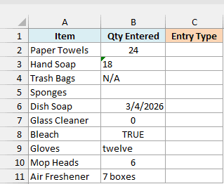
Below is a stock-count form, and I want to label each entry Number, Text, or Other in column C.

The entries mix quantities, text, a blank, a date, and logical TRUE.

Here is the formula:

=IF(ISNUMBER(B2:B11),"Number",IF(ISTEXT(B2:B11),"Text","Other"))

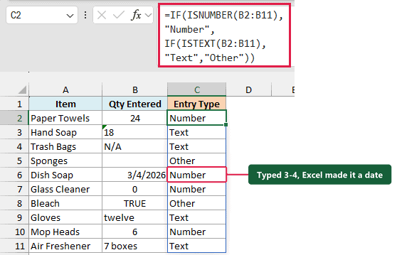
Here is how this formula works:

• ISNUMBER(B2:B11) checks each entry. The outer IF writes “Number” wherever that test returns TRUE.
• For the remaining entries, ISTEXT(B2:B11) checks for text. The inner IF writes “Text” when that test returns TRUE.
• If neither test passes, the inner IF writes “Other”. The results spill into C2:C11.

Glass Cleaner’s 0 gets Number, since zero is still a number. Hand Soap’s 18 gets Text because it was typed in as text.

The blank for Sponges and the TRUE for Bleach get Other, because they are neither numbers nor text.

ISNUMBER and ISTEXT aren’t opposites. Blanks and logical values fail both tests, as do errors, which is why the third label matters.

One more thing to watch for is Dish Soap. Someone typed 3-4, and Excel turned it into the date 3/4/2026, so the formula labels it Number.

Important: Dates and times return TRUE because Excel stores them as serial numbers. If your rule must exclude dates, ISNUMBER alone won’t do it.

You can read more about these tests in the IS functions guide, and about choosing labels in the IF function tutorial.

Example 3: Find Text with ISNUMBER and SEARCH

You can also use ISNUMBER to check whether a cell contains specific text.

Below is a meal-kit support ticket list, and I want to show Review in column C for every ticket whose summary contains the keyword in F1.

F1 holds the keyword refund.

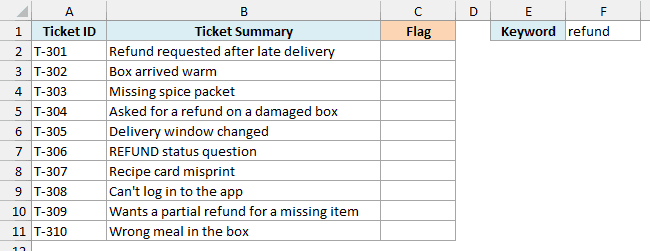
Here is the formula:

=IF($F$1="","",IF(ISNUMBER(SEARCH($F$1,B2:B11)),"Review",""))

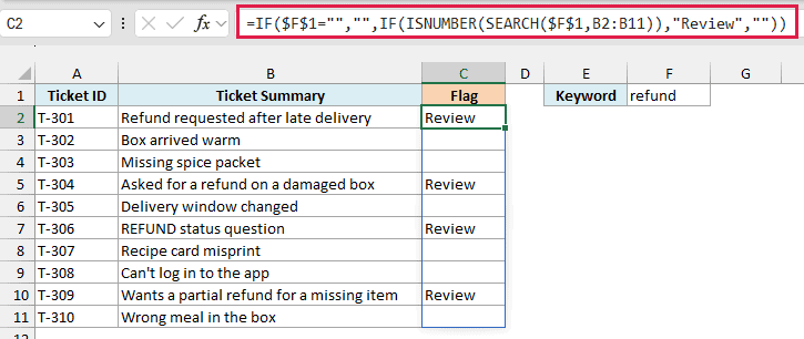
The results spill into C2:C11, and the four tickets that mention a refund show Review. The other cells look blank.

Here is how this formula works:

• SEARCH($F$1,B2:B11) looks for the keyword in each summary. It returns the keyword’s starting position when found, or #VALUE! when it isn’t found.
• ISNUMBER turns those results into TRUE or FALSE. A position number gives TRUE, while the error gives FALSE.
• The inner IF writes “Review” for TRUE and an empty string for FALSE.
• The outer IF checks F1 first. If the keyword cell is empty, it returns an empty string instead of checking the summaries.

Important: SEARCH returns 1 for an empty keyword. Without the outer IF, clearing F1 would mark every ticket for review.

The SEARCH function ignores case, so refund, Refund, and REFUND all match.

If you need a case-sensitive match, use the FIND function instead.

Note that ISNUMBER doesn’t check whether a cell contains digits. A summary like “Ticket 204” is still text, so ISNUMBER returns FALSE for it.

That’s why this formula works. ISNUMBER isn’t testing the summary itself, it’s testing the position number that SEARCH returns.

For more ways to check whether some text appears inside a cell, see the partial text matching guide.

Example 4: Highlight Text Entries with Conditional Formatting

Let’s use the same numeric check to spot entries that could disappear from a total.

Below is a café’s daily takings sheet, and I want to highlight filled cells that aren’t real numbers in column B.

I’ll use conditional formatting for this, so there’s no need for a helper column.

Some takings are text, including 985, “pending”, “1,420”, and “$960”. B7 is blank because the café was closed on 3/7/2026.

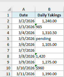
Here are the steps:

1. Select B2:B11.

2. Go to Home > Conditional Formatting > New Rule.

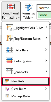
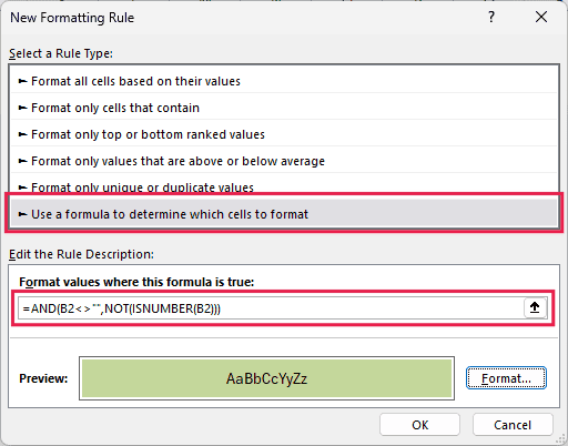
3. In the New Formatting Rule dialog, choose “Use a formula to determine which cells to format“.

4. Click Format, go to the Fill tab, pick a light green from the palette, and click OK.

5. In the formula box, enter this formula:

=AND(B2<>"",NOT(ISNUMBER(B2)))

6. Click OK.

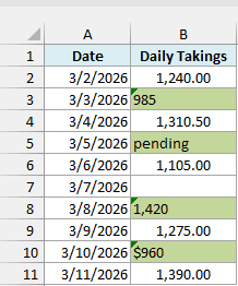
B3, B5, B8, and B10 get a light green fill. The blank B7 stays white.

Here is how this formula works:

• B2<>"" checks that the cell isn’t empty, so closed days don’t get highlighted.
• NOT(ISNUMBER(B2)) returns TRUE when the entry isn’t a number. Here, it catches the four text entries.
• AND requires both checks to pass before applying the fill.

B2 is a relative reference. As Excel applies the rule down B2:B11, each cell checks its own value.

Note that “1,420” and “$960” look like amounts, but they were typed in as text, which is why they get highlighted.

Important: SUM skips text in a range. These takings would silently drop out of your total, so convert the numeric text before adding up the days.

Example 5: Allow Only Numbers or TBD

Now let’s stop unwanted entries at the point where someone types them.

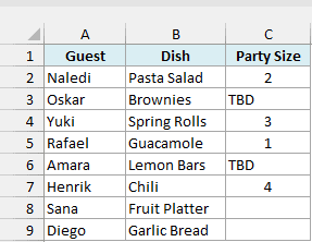
Below is a team potluck sign-up sheet, and I want column C to accept only numbers greater than 0 or the word TBD.

Party sizes already include numbers and TBD. Sana’s C8 and Diego’s C9 are still blank.

Here are the steps:

1. Select C2:C9.

2. Go to Data > Data Validation.

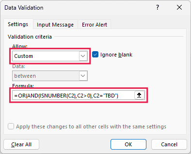
3. On the Settings tab, set Allow to Custom.

4. In the Formula box, enter this formula:

=OR(AND(ISNUMBER(C2),C2>0),C2="TBD")

5. Click OK.

Now, if someone types the word two in C8, Excel shows its standard stop alert and rejects the entry.

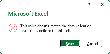
If you want a friendlier message that tells people what to type, you can add your own title and message on the Error Alert tab before clicking OK.

Here is how this formula works:

• ISNUMBER(C2) checks that the entry is a real number, and C2>0 checks that it is positive. AND requires both to pass.
• C2="TBD" allows the placeholder instead of a number. This comparison isn’t case sensitive, so tbd works too.
• OR accepts the entry when either the positive-number test or the TBD test passes.

The built-in Decimal option can check a numeric range, but it can’t also allow the word TBD. That’s why this needs a Custom rule.

Within this rule, the ISNUMBER function matters because Excel ranks text above numbers in comparisons. Without it, text such as abc would pass C2>0.

Also note that this rule accepts decimals like 2.5, as it only checks for a positive number, not a whole number.

To apply the same test to every entry, the formula refers to C2, not C2:C9. Data validation adjusts this relative reference to check each cell on its own.

For more on setting up these rules, see the data validation guide.

Example 6: COUNTIF ISNUMBER Alternative with a Condition

Now let’s count the entries that have numeric hours, but only for one shift.

Below is a volunteer hours sheet, and I want to count entries with numeric hours for the shift in F1, with the result in F2.

F1 holds Morning, so the count is for that shift.

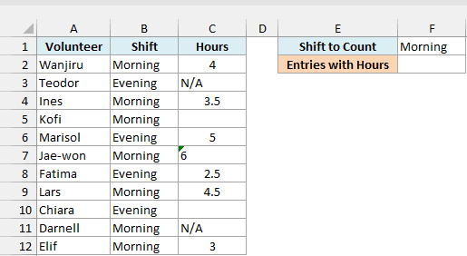
Here is the formula:

=SUM(ISNUMBER(C2:C12)*(B2:B12=F1))

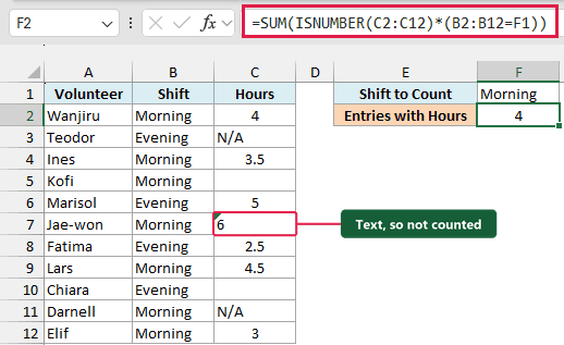
This returns 4, for Wanjiru, Ines, Lars, and Elif. Jae-won’s 6 is text, so it doesn’t count, even though the shift is Morning.

Here is how this formula works:

• ISNUMBER(C2:C12) returns TRUE or FALSE for each Hours cell.
• B2:B12=F1 returns TRUE or FALSE depending on whether the shift matches Morning in F1.
• Multiplying the two sets of results converts TRUE/FALSE into 1/0. A row gives 1 only when both checks are TRUE.
• SUM adds those 1s, giving the number of matching entries rather than the total hours.

You can’t use ISNUMBER as the criteria in COUNTIF, which is why this formula multiplies the two checks and adds them up with SUM instead.

Pro Tip: For a plain count of all numeric Hours cells, use COUNT. =COUNT(C2:C12) returns 6 here, across both shifts.

If you are using Excel 2019 or earlier, the SUM formula above needs Ctrl+Shift+Enter. To avoid that, enter the below formula in cell F2 instead:

=SUMPRODUCT(ISNUMBER(C2:C12)*(B2:B12=F1))

It also returns 4.

Example 7: Check Whether IDs Exist in Another List

You can also turn a lookup result into a yes-or-no check.

Below are eight gym class sign-ups and a member register, and I want TRUE for registered IDs and FALSE for missing IDs in column B.

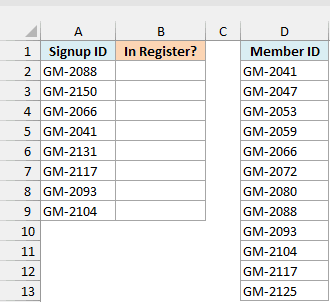
Here is the formula:

=ISNUMBER(XMATCH(A2:A9,D2:D13))

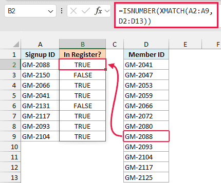
The results spill into B2:B9.

GM-2150 and GM-2131 return FALSE because neither appears in the register. The other six IDs return TRUE.

Here is how this formula works:

• XMATCH(A2:A9,D2:D13) searches the register for each signup ID. It uses an exact match by default.
• When it finds an ID, XMATCH returns its position in the register. When it doesn’t, it returns #N/A.
• ISNUMBER converts each position into TRUE and each #N/A into FALSE.

Notice that the IDs themselves are text. ISNUMBER is testing the position returned by XMATCH, not whether an ID is numeric.

XMATCH is available in Microsoft 365, Excel 2021 or later, and Excel for the web.

If you are using Excel 2019 or earlier, enter the below formula in cell B2 and then copy it down to B9:

=ISNUMBER(MATCH(A2,$D$2:$D$13,0))

The 0 tells the MATCH function to look for an exact match, so it checks for the same ID.

Example 8: Extract Rows with FILTER and ISNUMBER

For the last example, let’s pull out the rows that hold real numbers.

Below is a run log, and I want to extract the dates and distances for completed runs into columns D and E.

The distance column has numeric distances, but also Rest, Rained out, and a blank cell.

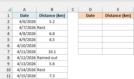
Here is the formula:

=FILTER(A2:B11,ISNUMBER(B2:B11),"No runs logged")

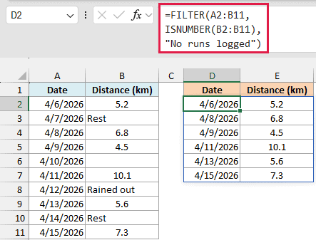
The result spills across D2:E7, giving six runs. Rest days, Rained out, and the blank distance don’t appear.

Here is how this formula works:

• ISNUMBER(B2:B11) returns TRUE for each numeric distance and FALSE for the text and blank entries.
• FILTER keeps the rows from A2:B11 where that test is TRUE, bringing back both the date and the distance.
• "No runs logged" is the fallback message if no distance qualifies.

Important: The FILTER function returns stored serial numbers, so unformatted results look like numbers. Format the output date cells in column D as dates.

The FILTER function needs Microsoft 365, Excel 2021 or later, or Excel for the web.

In this article, I showed you how to use ISNUMBER to check entries and combine it with other functions to count matches or filter rows.

I hope you found this article helpful.

List of All Excel Functions

Other Excel Articles You May Also Like:

• COUNTIF Function in Excel
• IFERROR Function in Excel
• How to Count Cells that Contain Text Strings
• COUNT vs COUNTA in Excel: What’s the Difference?
• Count Cells That Are Not Blank in Excel
• 20 Advanced Excel Functions and Formulas (for Excel Pros)
• How to use ISBLANK in Excel