

The DEC2BIN function in Excel converts a regular decimal number into binary, the number system that uses only 0s and 1s. So 13 becomes 1101, and 255 becomes 11111111.
It’s handy when you’re checking binary homework, or when you need numbers in a fixed-width binary format and don’t want to work them out by hand.
There are two catches. DEC2BIN only converts numbers from -512 to 511, and it doesn’t accept a whole range, so a formula like =DEC2BIN(B2:B11) returns an error instead of a list of results.
In this article, I’ll show you how to use DEC2BIN with six practical examples, including how to convert a whole list in one go and what to use for numbers above 511.
Follow along with the example file
DEC2BIN Function Examples.xlsx
DEC2BIN Function Syntax
Here is the syntax of the DEC2BIN function:
=DEC2BIN(number, [places])
- number – The decimal number you want to convert. It must be a number from -512 to 511, or a reference to a cell that holds one.
- places – (Optional) The number of characters you want in the result. DEC2BIN adds zeros on the left of a positive result to reach this length.
If you leave out places, DEC2BIN uses only as many digits as the number needs. So 5 comes back as 101, and 255 comes back as 11111111.
When you give places, a positive result is padded with leading zeros, so =DEC2BIN(9,6) returns 001001. This is useful when you want every result in a column to have the same number of digits.
If places is smaller than the number of digits a positive result needs, DEC2BIN returns the #NUM! error. For example, 9 is 1001 in binary, so =DEC2BIN(9,3) returns #NUM!.
You also get #NUM! when places is 0, negative, or more than 10.
Negative numbers work a little differently. A places value from 1 to 10 doesn’t shorten them, so they always come back as 10 digits (Example 4 shows why).
If the number has decimals, DEC2BIN drops them without rounding, so 9.9 is converted as 9. Text that isn’t a number, like “abc”, returns the #VALUE! error.
The DEC2BIN function works in all Excel versions, including Excel 365, 2024, 2021, 2019, 2016, and Excel for Mac.
When to Use the DEC2BIN Function
Use this function when you need to:
- Convert decimal numbers into binary
- Show binary values with a fixed number of digits by adding leading zeros
- Get the binary form of negative numbers
- Turn values that come from other functions, like the hours and minutes of a time, into binary
Let me show you a few practical examples of how to use the DEC2BIN function in Excel.
Example 1: Convert Decimal to Binary in Excel
Let’s start with a simple example.
Below is the answer key for a worksheet where students convert numbers into binary, and I want the binary answer for each number in column C.
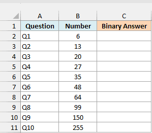
Here is the formula I entered in cell C2 and then copied down to C11:
=DEC2BIN(B2)
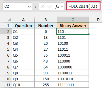
DEC2BIN takes the number in B2 and returns it in binary, so 6 becomes 110. As you copy the formula down, B2 changes to B3, B4, and so on, so every question gets its own answer.
In case you’re wondering how 13 becomes 1101, each place in a binary number is worth double the place to its right. From the right, the places are worth 1, 2, 4, 8, and so on.
13 is 8 + 4 + 1, so the 8, 4, and 1 places get a 1, and the 2 place gets a 0. That gives you 1101.
The results are text, which is why they line up on the left side of the cells. That’s also what lets DEC2BIN keep leading zeros, which you’ll see in Example 3.
You might expect =DEC2BIN(B2:B11) to convert the whole list in one go, but it returns the #VALUE! error. Example 2 shows a simple way to make it work.
Example 2: Convert a Whole List With One Formula
Now let’s convert an entire list with a single formula.
Below is a list of players on a basketball team with their jersey numbers, and I want each jersey number in binary in column C.
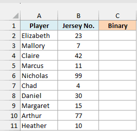
Here is the formula:
=DEC2BIN(+B2:B11)
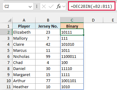
This is the =DEC2BIN(B2:B11) formula from the end of Example 1 with one change, a plus sign before the range. Without the plus sign, DEC2BIN returns #VALUE!, because it’s one of the older Excel functions that can’t take a range reference.
The plus sign makes Excel work out +B2:B11 first, which turns the range into a list of values. DEC2BIN can handle a list, so it converts every jersey number, and the results spill into C2:C11 on their own.
This same plus-sign trick works for other functions that won’t spill, such as EOMONTH and EDATE.
If you are using Excel 2019 or earlier, enter the below formula in cell C2 and then copy it down to C11:
=DEC2BIN(B2)
Example 3: Add Leading Zeros With the Places Argument
If you look at the results in Example 2, the binary numbers all have different lengths. Jersey 7 is just 111, while jersey 99 is 1100011.
Below is the same team list, and this time I want every jersey number as a 7-digit binary value in column D.
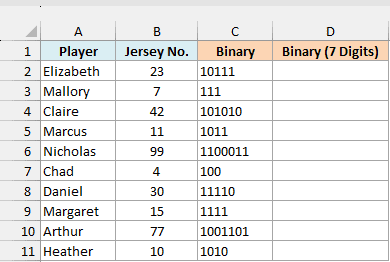
Here is the formula:
=DEC2BIN(+B2:B11,7)
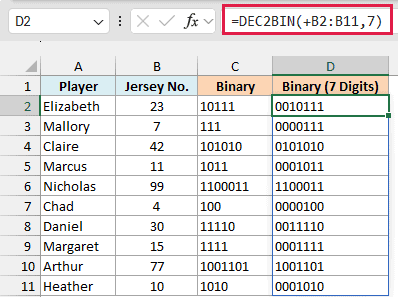
The 7 at the end is the places argument. It tells DEC2BIN to return 7 characters, so it adds zeros on the left of any shorter result.
Jersey 7 now shows as 0000111, and jersey 23 shows as 0010111.
I picked 7 because the biggest jersey number, 99, needs 7 binary digits. If I had used 6, the two 7-digit jerseys, 99 (Nicholas) and 77 (Arthur), would return #NUM!, because they can’t fit in 6 characters.
Pro Tip: To find how many digits your biggest number needs, use =LEN(DEC2BIN(MAX(B2:B11))). Here it returns 7, so 7 is the smallest places value that works for the whole list.
If you are using Excel 2019 or earlier, enter the below formula in cell D2 and then copy it down to D11:
=DEC2BIN(B2,7)
Example 4: Convert Negative Numbers to Binary
This next one can look a little strange at first, because negative numbers come back as long strings of 1s.
Below are the lowest temperatures (in °F) recorded on ten January days in a cold city, and I want each one as a 10-digit binary value in column C.
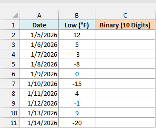
Here is the formula:
=DEC2BIN(+B2:B11,10)
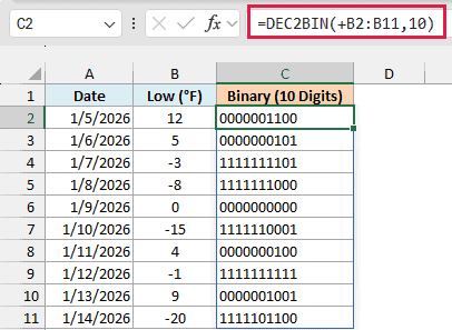
For a negative number, DEC2BIN always returns 10 digits, and the first digit is always 1. So -3 comes back as 1111111101, and -1 comes back as 1111111111.
These negative values use a system called two’s complement. Ten binary digits give you 1,024 different patterns, and a negative number gets the pattern you reach by counting back from 1,024.
So -3 gets the pattern for 1,021 (1,024 minus 3). You can check it with =BASE(1021,2), which returns 1111111101 (the BASE function is covered in Example 5).
I used 10 for places so the positive temperatures also show all 10 digits. Now every positive value starts with 0 and every negative value starts with 1, so the first digit tells you the sign.
That’s also where the -512 to 511 limit comes from. With 10 digits and the first one used for the sign, the smallest value is 1000000000 (-512) and the largest is 0111111111 (511).
Note that places doesn’t change negative results. Even =DEC2BIN(-3,4) returns all 10 digits instead of an error, so you can’t shorten a negative result.
If you are using Excel 2019 or earlier, enter the below formula in cell C2 and then copy it down to C11:
=DEC2BIN(B2,10)
Example 5: DEC2BIN vs BASE for Numbers Above 511
Since DEC2BIN stops at 511, you need a different function for bigger numbers.
Below is a list of menu items with their calories, and I want each calorie count in binary, first with DEC2BIN in column C and then with the BASE function in column D.
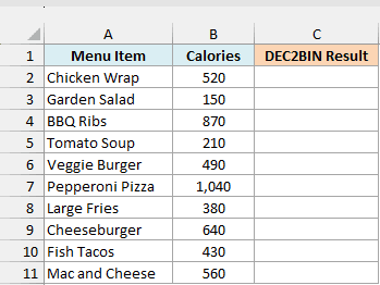
Here is the DEC2BIN formula:
=DEC2BIN(+B2:B11)
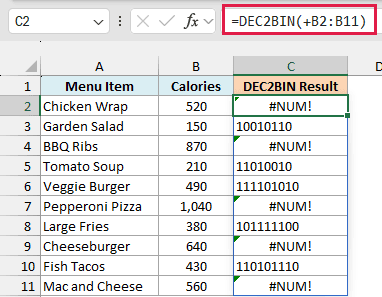
Every value up to 511 converts fine, like the Garden Salad’s 150 and the Veggie Burger’s 490. But the five items above 511, such as the Chicken Wrap with 520 calories, return #NUM!.
Now here is the BASE formula in column D:
=BASE(B2:B11,2)
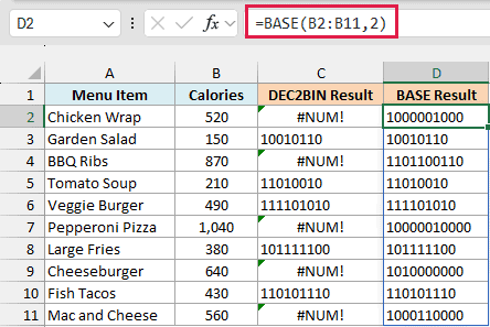
The BASE function converts a number into any number system, and the 2 tells it to use binary. It converts every calorie count, including 1,040 for the Pepperoni Pizza, which becomes 10000010000.
BASE also takes the range directly, so you don’t need the plus sign here. It’s available in Excel 2013 and later versions.
Important: BASE doesn’t work with negative numbers and returns #NUM! for them. So use BASE for positive numbers that can go above 511, and stick with DEC2BIN when your list has negative values.
If you are using Excel 2019 or earlier, enter the below formula in cell C2 and then copy it down to C11:
=DEC2BIN(B2)
Then enter the below formula in cell D2 and copy it down to D11:
=BASE(B2,2)
Example 6: Show Times as a Binary Clock
Let’s finish with a fun one, where DEC2BIN works together with a couple of other functions.
Below is a list of train departure times, and I want to show each time the way a binary clock would, with the hours and minutes in binary, in column C.
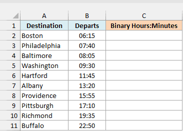
Here is the formula:
=DEC2BIN(HOUR(B2:B11),5)&":"&DEC2BIN(MINUTE(B2:B11),6)
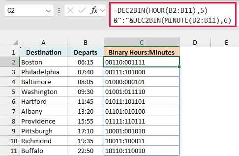
How this formula works:
- HOUR(B2:B11) gets the hour from each departure time, on the 24-hour clock. So the Pittsburgh train at 17:10 gives 17.
- DEC2BIN(…,5) converts each hour into a 5-digit binary value. Five digits are enough for every hour from 0 to 23, so 17 becomes 10001.
- MINUTE(B2:B11) gets the minutes, and DEC2BIN(…,6) converts them into 6 digits, which covers every minute from 0 to 59. So 10 becomes 001010.
- The & operator joins the two parts with a colon in between, so 17:10 becomes 10001:001010.
Notice there’s no plus sign in this formula. HOUR and MINUTE already return a list of numbers instead of a range, so DEC2BIN accepts them as they are.
If you are using Excel 2019 or earlier, enter the below formula in cell C2 and then copy it down to C11:
=DEC2BIN(HOUR(B2),5)&":"&DEC2BIN(MINUTE(B2),6)
So that’s how you can use the DEC2BIN function in Excel to turn decimal numbers into binary, one at a time or a whole list at once. Just keep the -512 to 511 limit in mind, and switch to BASE when your numbers get bigger.
If you need hexadecimal or octal instead, Excel has the DEC2HEX and DEC2OCT functions. And to turn binary back into a decimal number, use the BIN2DEC function or the DECIMAL function.
I hope you found this tutorial useful.
Other Excel Articles You May Also Like:
