How to Compare Two Columns in Excel (for matches & differences)

The one query that I get a lot is – ‘how to compare two columns in Excel?’.

This can be done in many different ways, and the method to use will depend on the data structure and what the user wants from it.

For example, you may want to compare two columns and find or highlight all the matching data points (that are in both the columns).

Or you may want only the differences (where a data point is in one column and not in the other), etc.

Since I get asked about this so much, I decided to write this massive tutorial with an intent to cover most (if not all) possible scenarios.

In this tutorial, I’ll show you how to compare two columns row by row, highlight matches and differences, find missing values, and pull matching data.

If you find this useful, do pass it on to other Excel users.

Note that the techniques to compare columns shown in this tutorial are not the only ones.

Based on your dataset, you may need to change or adjust the method. However, the basic principles would remain the same.

If you think there is something that can be added to this tutorial, let me know in the comments section.

Compare Two Columns For Exact Row Match

This one is the simplest form of comparison. In this case, you need to do a row by row comparison and identify which rows have the same data and which ones do not.

Below is a data set where I need to check whether the name in column A (Name in CRM) is the same in column B (Name on Invoice) or not.

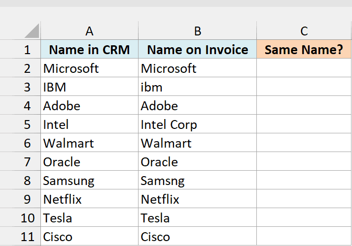
If there is a match, I need the result as “TRUE”, and if it doesn’t match, then I need the result as “FALSE”.

The below formula would do this:

=A2:A11=B2:B11

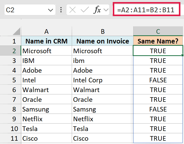
Enter this formula in cell C2, and it spills down automatically for all the rows.

It compares each name in column A with the name in the same row in column B. Intel and Samsung return FALSE because the invoice says “Intel Corp” and “Samsng”.

Spilling formulas like this one work in Microsoft 365 and Excel 2021 or later. In older versions, use =A2=B2 in cell C2 and copy it down.

If you want to get a more descriptive result, you can use a simple IF formula to return “Match” when the names are the same and “Mismatch” when the names are different.

=IF(A2:A11=B2:B11,"Match","Mismatch")

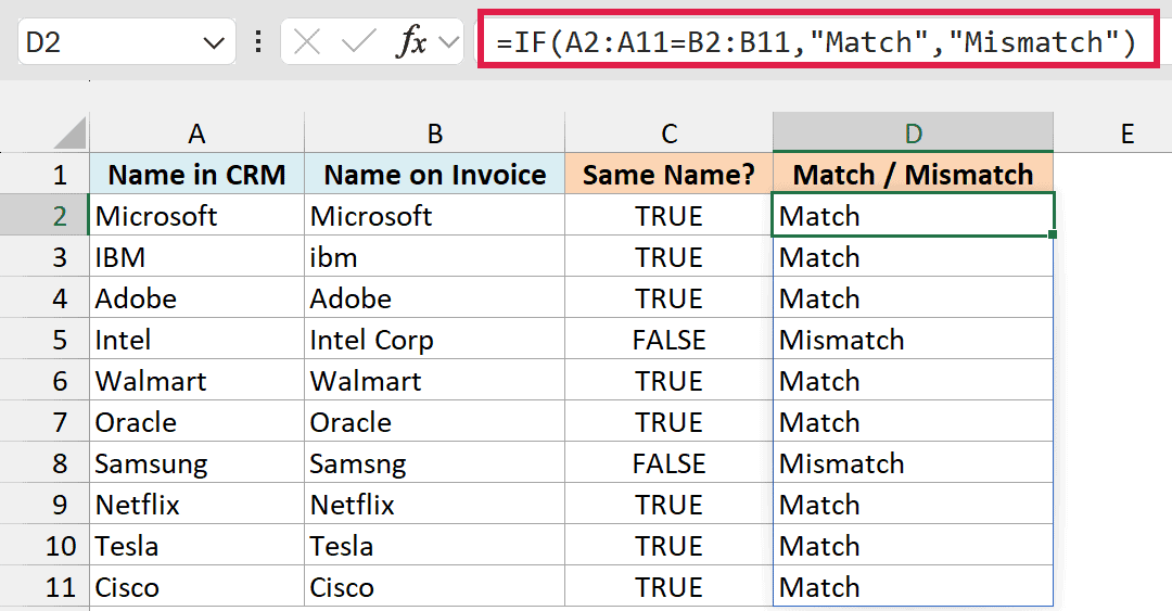
Enter this formula in cell D2. In older versions of Excel, use =IF(A2=B2,"Match","Mismatch") and copy it down.

Note that both these formulas are not case sensitive. So ‘IBM’ in column A and ‘ibm’ in column B are treated as a match.

In case you want to make the comparison case sensitive, use the following IF formula:

=IF(EXACT(A2:A11,B2:B11),"Match","Mismatch")

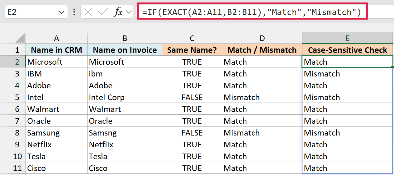
With the above formula, ‘IBM’ and ‘ibm’ would be considered two different names and the above formula would return ‘Mismatch’.

Enter this formula in cell E2. In older versions of Excel, use =IF(EXACT(A2,B2),"Match","Mismatch") and copy it down.

The EXACT function checks whether two text values are exactly the same, including the case of every letter.

If you need more ways to compare text in Excel, I have a separate tutorial on that.

Highlight Row Differences Using Go To Special (Ctrl + \)

If all you want is to quickly spot the rows where the two columns are different, you don’t need a formula at all.

Excel has a built-in Row Differences option that selects every cell that doesn’t match the other column in its row. You can then give those cells a fill color.

Below I have the same dataset with names in column A (Name in CRM) and column B (Name on Invoice).

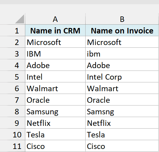
Here are the steps to highlight the row differences:

1. Select the names in both columns (A2:B11 in this example). Start the selection from cell A2, so column A is the column Excel compares against.

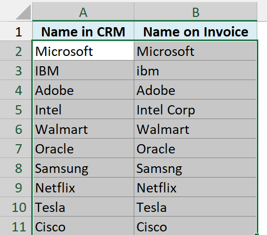
2. Press Ctrl + \ (the backslash key). This selects the cells in column B that are different from column A in the same row.

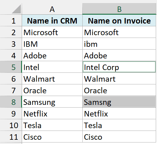
3. Click the Home tab, click the Fill Color drop-down, and pick a color.

This highlights ‘Intel Corp’ and ‘Samsng’, the two names that don’t match the name in column A.

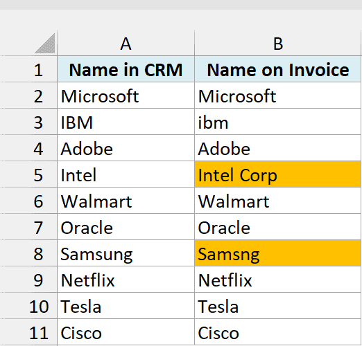
If the shortcut doesn’t work on your keyboard, go to Home > Find & Select > Go To Special, select Row differences, and click OK. It does the same thing.

Like the equal to operator, Row Differences is not case sensitive, so it doesn’t flag ‘IBM’ and ‘ibm’.

Also note that this is a one-time highlight, so it won’t update if you change the data later.

Highlight Rows with Matching Data (or Different Data)

If you want to highlight the rows that have matching data (instead of getting the result in a separate column), you can do that by using Conditional Formatting.

Unlike the Row Differences method, conditional formatting stays live. If you change a name, the highlight updates on its own.

Below I have the dataset with names in column A (Name in CRM) and column B (Name on Invoice), and I want to highlight the rows where both names are the same.

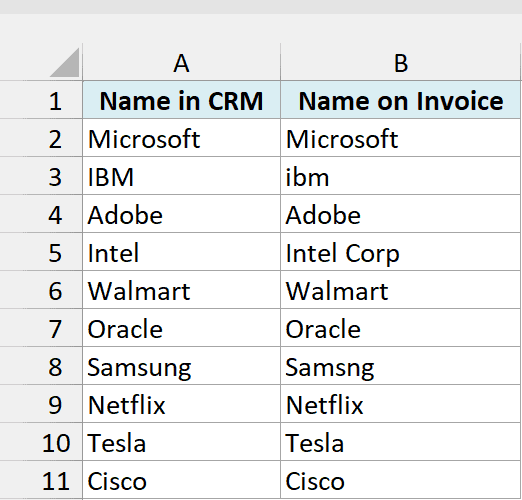
Here are the steps to do this:

1. Select the entire dataset (without the headers). In this example, that’s A2:B11.

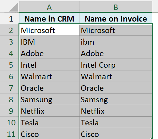
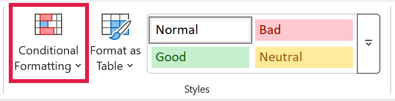
2. Click the ‘Home’ tab.

3. In the Styles group, click on the ‘Conditional Formatting’ option.

4. From the drop-down, click on ‘New Rule’.

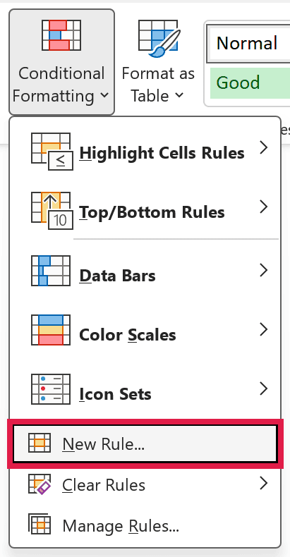
5. In the ‘New Formatting Rule’ dialog box, click on the ‘Use a formula to determine which cells to format’.

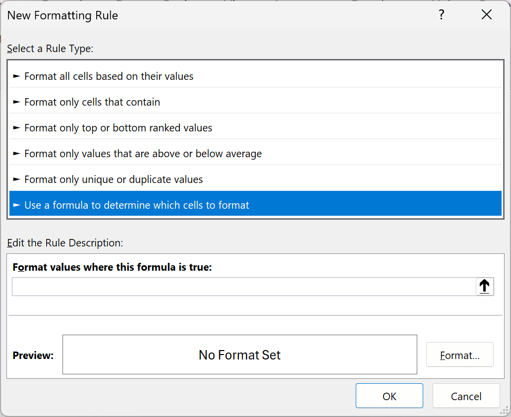
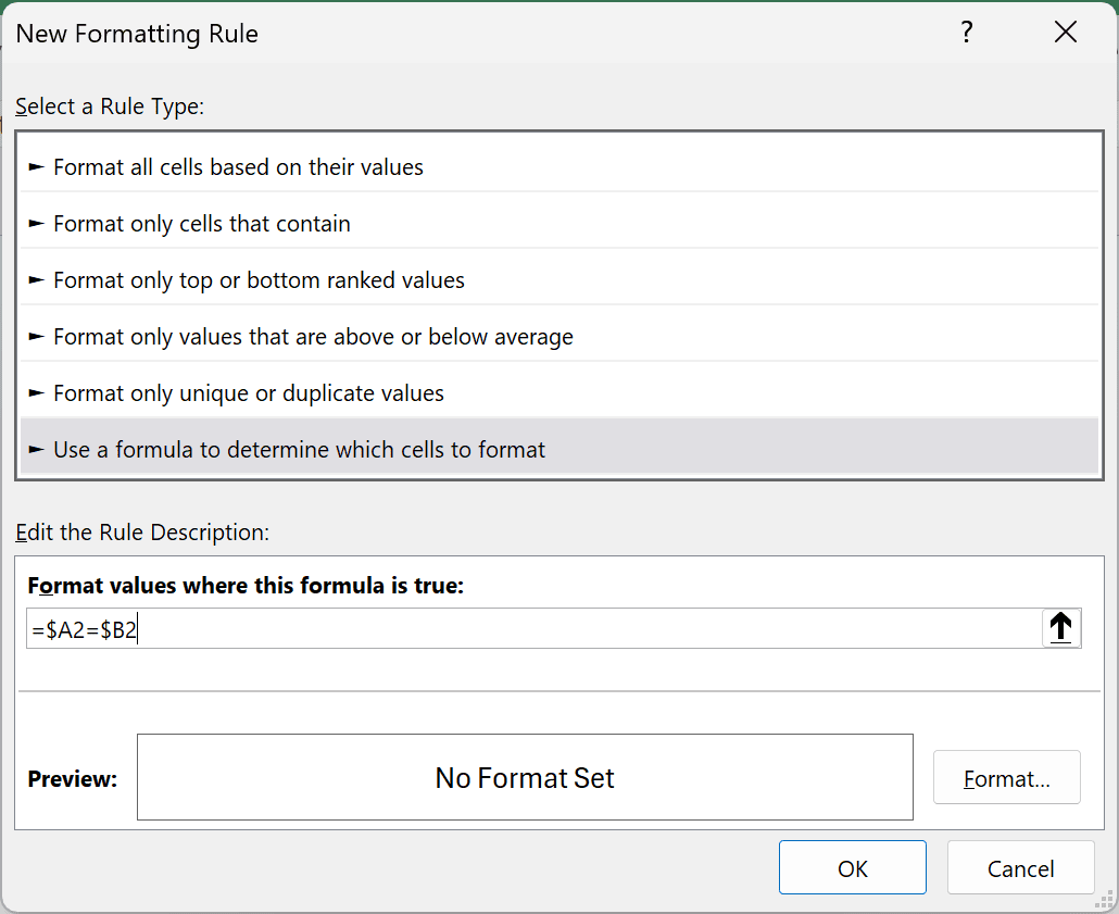
6. In the formula field, enter the formula: =$A2=$B2

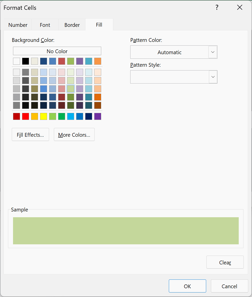
7. Click the Format button and specify the format you want to apply to the matching cells.

8. Click OK.

This will highlight all the cells where the names are the same in each row.

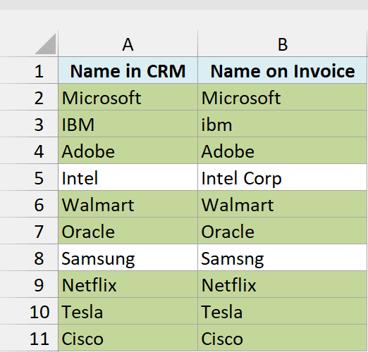
The dollar sign in $A2 and $B2 locks the columns but not the row. So every cell in row 2 checks A2 against B2, every cell in row 3 checks A3 against B3, and so on.

Make sure the row number in the formula (2 here) is the first row of your selection. If you select from row 1, use =$A1=$B1 instead.

If you want to highlight the rows where the names are different, follow the same steps, but use this formula in step 6:

=$A2<>$B2

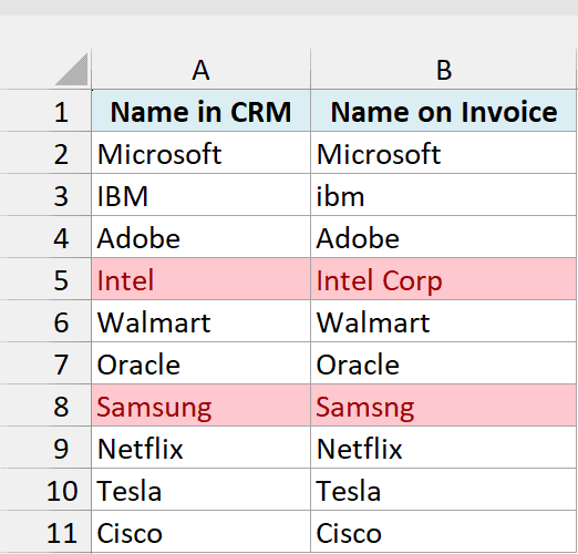
The <> operator means ‘not equal to’, so only the rows for Intel and Samsung get highlighted.

Compare Two Columns and Highlight Matches

If you want to compare two columns and highlight matching data, you can use the duplicate functionality in conditional formatting.

Note that this is different than what we have seen when comparing each row. In this case, we will not be doing a row by row comparison.

Often, you’ll get datasets where there are matches, but these may not be in the same row.

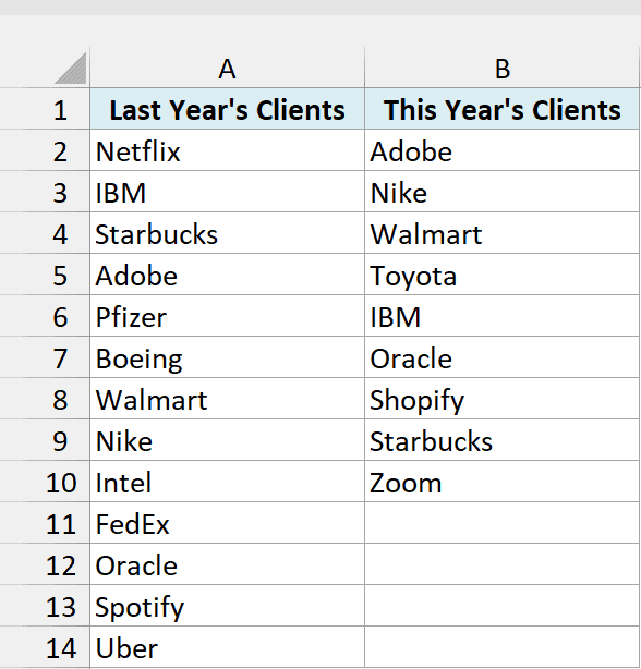
Something as shown below, where I have last year’s clients in column A and this year’s clients in column B:

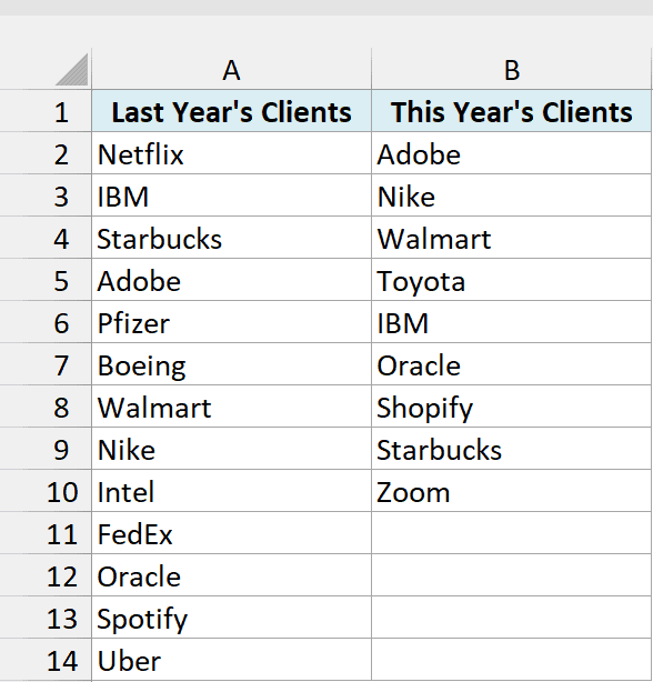
Note that the list in column A is bigger than the one in B. Also some names are there in both the lists, but not in the same row (such as IBM, Adobe, Walmart).

If you want to highlight all the matching company names, you can do that using conditional formatting.

Here are the steps to do this:

1. Select the entire data set (A2:B14 in this example).

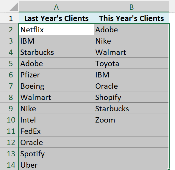
2. Click the Home tab, and in the Styles group, click on the ‘Conditional Formatting’ option.

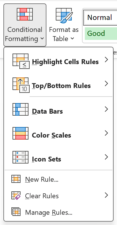
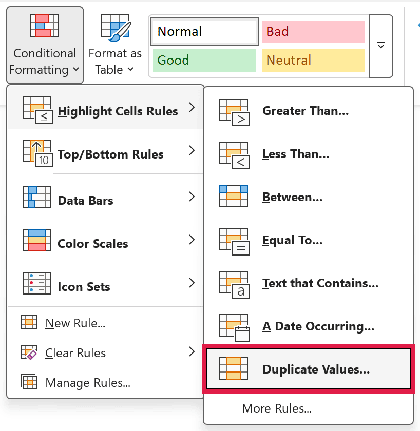
3. Hover the cursor on the Highlight Cells Rules option, and click on Duplicate Values.

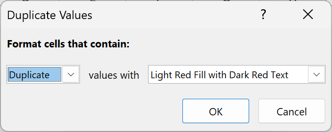
4. In the Duplicate Values dialog box, make sure ‘Duplicate’ is selected.

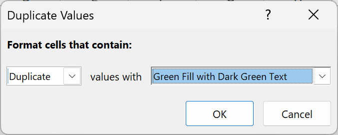
5. Specify the formatting. I’ve picked ‘Green Fill with Dark Green Text’.

6. Click OK.

The above steps would give you the result as shown below.

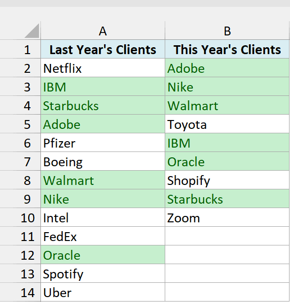
All six names that appear in both lists get highlighted, no matter which row they are in. Excel ignores the empty cells at the bottom of column B.

Note: Conditional Formatting duplicate rule is not case sensitive. So ‘Apple’ and ‘apple’ are considered the same and would be highlighted as duplicates.

Important: This rule also highlights a name that appears twice in the same list, even when it’s not in the other list.

If your lists can have repeats like that, use a formula rule instead. Select A2:A14 and create a ‘Use a formula’ rule (same as the previous section) with this formula:

=ISNUMBER(MATCH(A2,$B$2:$B$10,0))

This highlights a name in column A only when it’s found in column B.

And if you only want to find duplicates within one list, I have a separate tutorial on that.

Compare Two Columns and Highlight Differences

In case you want to highlight the names which are present in one list and not the other, you can use the conditional formatting for this too.

Below I have the same two lists, with last year’s clients in column A and this year’s clients in column B.

Here are the steps to highlight the differences:

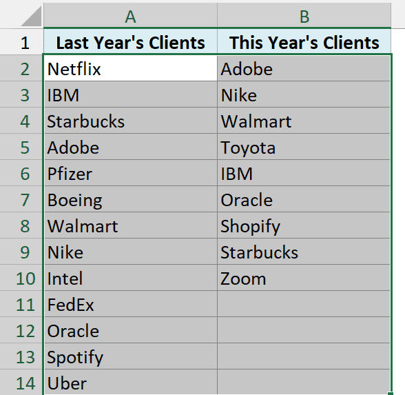
1. Select the entire data set (A2:B14).

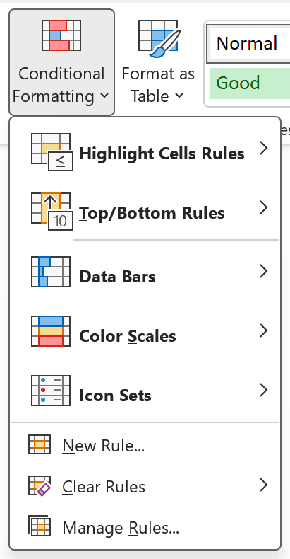
2. Click the Home tab, and in the Styles group, click on the ‘Conditional Formatting’ option.

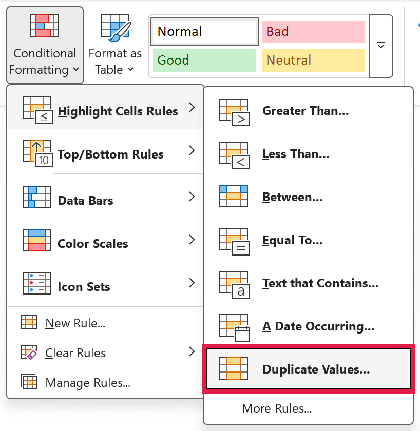
3. Hover the cursor on the Highlight Cells Rules option, and click on Duplicate Values.

4. In the Duplicate Values dialog box, make sure ‘Unique’ is selected.

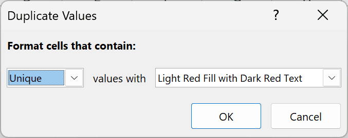
5. Specify the formatting. I’ve kept the default ‘Light Red Fill with Dark Red Text’.

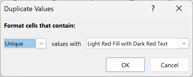
6. Click OK.

This will give you the result as shown below. It highlights all the cells that have a name that is not present on the other list.

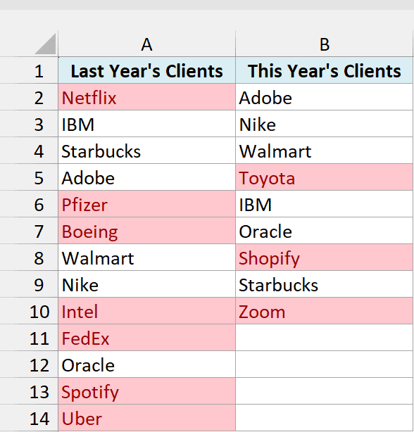
So you get the seven clients from last year that are missing this year, and also the three new clients this year (Toyota, Shopify, and Zoom).

Compare Two Columns and Find Missing Data Points

If you want to identify whether a data point from one list is present in the other list, you need to use the lookup formulas.

Suppose you have a dataset as shown below and you want to identify companies that are present in column A but not in column B.

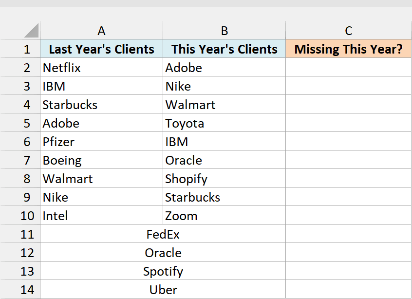
Below is the formula that will do this:

=ISNA(XMATCH(A2:A14,B2:B10))

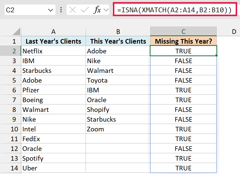
Enter this formula in cell C2, and it spills down for all 13 names in column A.

It returns TRUE for the companies that are missing in column B, and FALSE for the ones that are there.

How this formula works:

• XMATCH(A2:A14,B2:B10) looks for each company name from column A in column B. If it finds it, it returns its position in column B, else it returns a #N/A error.
• ISNA(…) returns TRUE when the result is the #N/A error and FALSE when it isn’t. So the names which return TRUE are the ones that are missing in column B.

XMATCH works in Microsoft 365 and Excel 2021 or later. In older versions, use this formula in cell C2 and copy it down:

=ISNA(MATCH(A2,$B$2:$B$10,0))

If you’re more used to VLOOKUP, =ISERROR(VLOOKUP(A2,$B$2:$B$10,1,0)) gives you the same TRUE/FALSE result.

This formula uses VLOOKUP to check whether a company name in A is present in column B or not.

If it is present, it will return that name from column B, else it will return a #N/A error.

ISERROR then returns TRUE when the VLOOKUP result is an error, and FALSE when it isn’t.

Note: Personally, I prefer using the Match function (or the combination of INDEX/MATCH) instead of VLOOKUP.

I find it more flexible and powerful. You can read the difference between Vlookup and Index/Match here.

If you want to get a list of all the names where there is no match, you can filter the result column to get all cells with TRUE.

Or you can get that list with a formula, which is what I cover next.

Get a List of Missing or Matching Values Using FILTER

The previous formula tells you which names are missing, but you still have to filter for them.

With the FILTER function, you can pull the list of missing names (or matching names) into a separate column with one formula.

Below I have the same two lists, and I want a list of last year’s clients that are not in this year’s list.

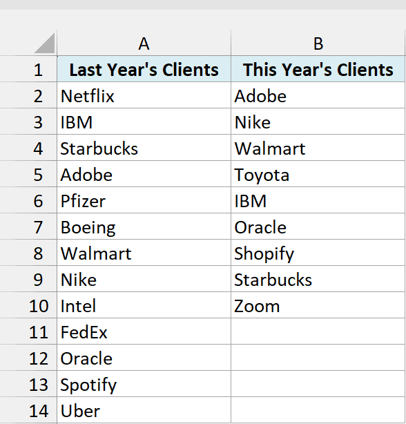
Here is the formula that will give us the result:

=FILTER(A2:A14,ISNA(XMATCH(A2:A14,B2:B10)))

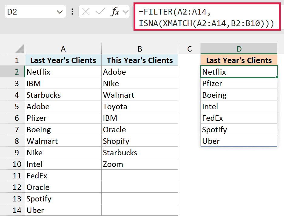
Enter it in cell D2, and it spills the seven missing names (Netflix, Pfizer, Boeing, Intel, FedEx, Spotify, and Uber).

The ISNA(XMATCH(…)) part is the same check from the previous section, and it returns TRUE for every missing name.

FILTER then keeps only the names from column A where that check is TRUE.

If you want the names that are in both lists instead, swap ISNA for ISNUMBER:

=FILTER(A2:A14,ISNUMBER(XMATCH(A2:A14,B2:B10)))

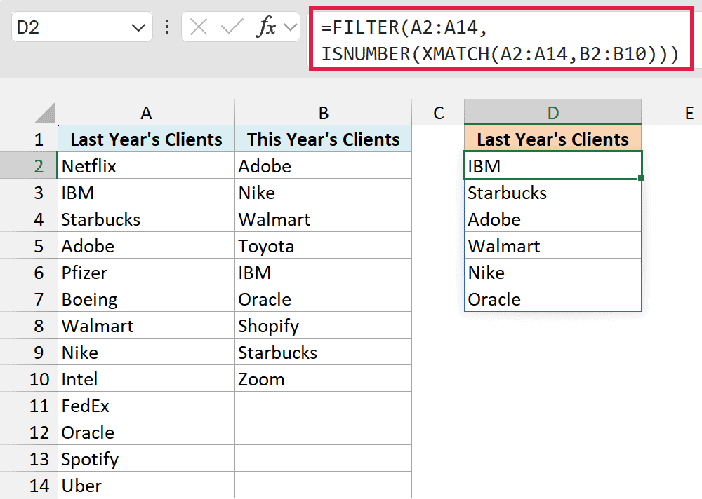
This returns the six clients that appear in both lists: IBM, Starbucks, Adobe, Walmart, Nike, and Oracle.

If there’s a chance that nothing matches, add a third argument such as “None found” to FILTER. Otherwise, the formula returns a #CALC! error when there’s nothing to show.

FILTER and XMATCH work in Microsoft 365 and Excel 2021 or later.

Compare Two Columns and Pull the Matching Data

If you have two datasets and you want to compare items in one list to the other and fetch the matching data point, you need to use the lookup formulas.

For example, in the below dataset, I have company names and their market values in columns A and B (these are sample values, not live numbers).

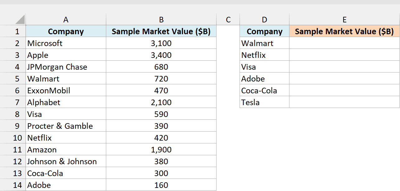
I want to fetch the market value for each company in column D. To do this, I need to look up that name in column A and then fetch the corresponding market value from column B.

Below is the formula that will do this:

=XLOOKUP(D2:D7,A2:A14,B2:B14,"Not found")

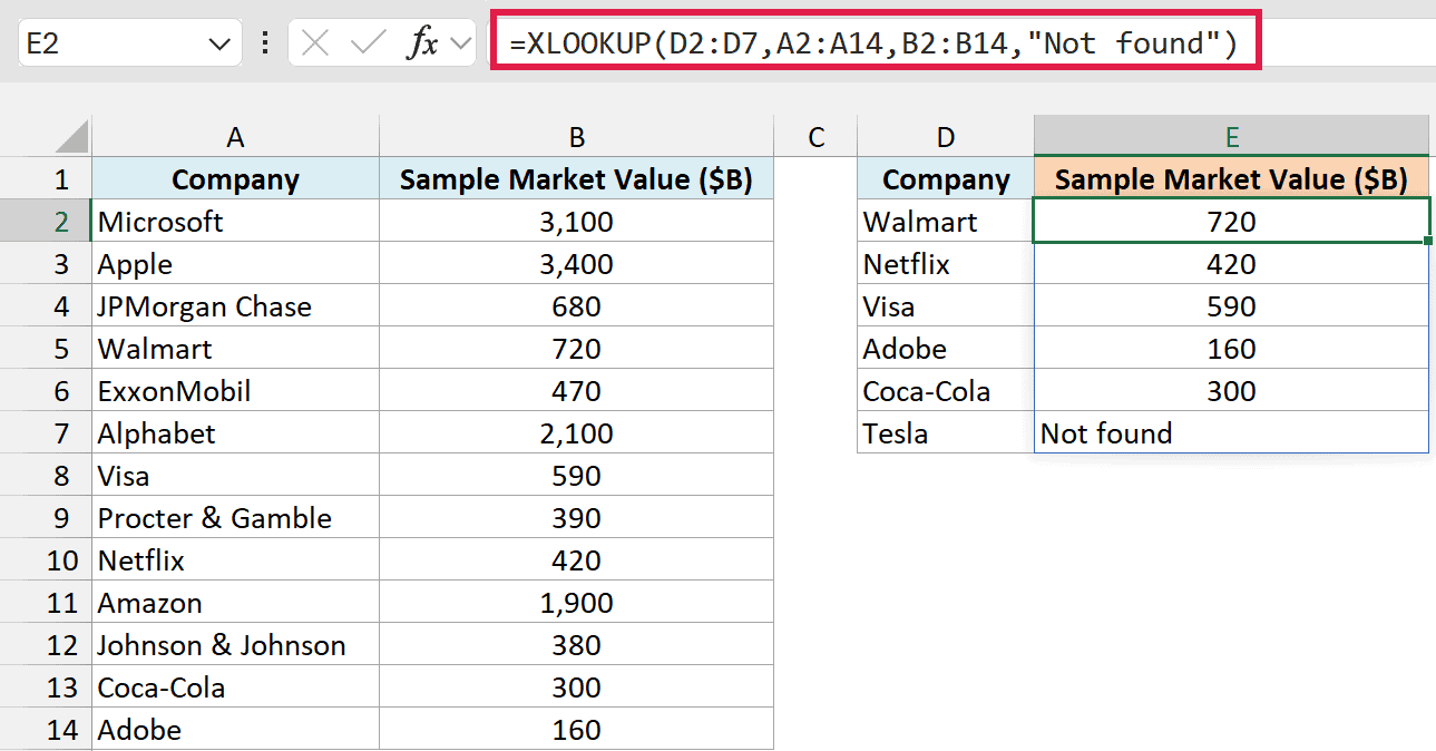
Enter this formula in cell E2, and it spills the market value for all six companies in column D.

The XLOOKUP function looks for each name from D2:D7 in A2:A14 and returns the value from the same row in B2:B14.

Tesla isn’t in the table, so XLOOKUP returns “Not found” (the fourth argument) instead of a #N/A error.

XLOOKUP works in Microsoft 365 and Excel 2021 or later. If you’re using an older version, use either of these formulas in cell E2 and copy it down:

=VLOOKUP(D2,$A$2:$B$14,2,0)

=INDEX($A$2:$B$14,MATCH(D2,$A$2:$A$14,0),2)

Both return a #N/A error for Tesla, since it isn’t in the table. Here is my guide on the VLOOKUP formula if you want to learn more about it.

If you’re not sure which one to use, here’s how VLOOKUP and XLOOKUP compare.

Pull the Matching Data Using a Partial Match (Wildcards)

In case you get a dataset where there is a minor difference in the names in the two columns, using the above-shown lookup formulas is not going to work.

These lookup formulas need an exact match to give the right result. There is an approximate match option in VLOOKUP or MATCH function, but that can’t be used here.

Suppose you have the data set as shown below.

Note that there are names that are not complete in column D (such as JPMorgan instead of JPMorgan Chase and Exxon instead of ExxonMobil).

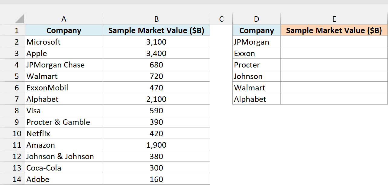
In such a case, you can use a partial lookup by using wildcard characters.

The following formula will give us the right result in this case:

=XLOOKUP("*"&D2:D7&"*",A2:A14,B2:B14,"Not found",2)

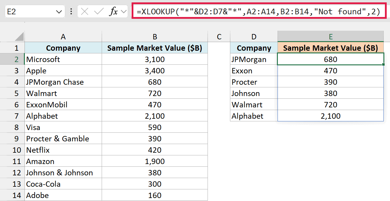
Enter it in cell E2, and it spills the market value for all six partial names.

In the above example, the asterisk (*) is a wildcard character that can represent any number of characters.

When the lookup value is flanked with it on both sides, any value in column A which contains the lookup value in column D would be considered as a match.

For example, Exxon would be a match for ExxonMobil (as * can represent any number of characters).

The 2 at the end is important. It tells XLOOKUP to treat the asterisk as a wildcard. Without it, XLOOKUP looks for the literal text Exxon and returns “Not found”.

In older versions of Excel, use either of these formulas in cell E2 and copy it down:

=VLOOKUP("*"&D2&"*",$A$2:$B$14,2,0)

=INDEX($A$2:$B$14,MATCH("*"&D2&"*",$A$2:$A$14,0),2)

VLOOKUP and MATCH accept wildcards in exact match mode by default, so they don’t need that extra argument.

Also, keep in mind that a partial match returns the first value that contains your text. So keep the partial names specific enough that they can only match one company.

So these are some of the ways you can compare two columns in Excel.

I hope you found this tutorial useful!

You May Also Like the Following Excel Tips & Tutorials:

• How to Compare Two Excel Sheets (for differences)
• How to Highlight Blank Cells in Excel.
• Highlight EVERY Other ROW in Excel.
• Excel Advanced Filter: A Complete Guide with Examples.
• Highlight Rows Based on a Cell Value in Excel
• How to Compare Dates in Excel (Greater/Less Than, Mismatches)
• Compare Two Lists (Free Online Tool)
• Apply Conditional Formatting Based on Another Column in Excel
• How to make VLOOKUP Case Sensitive