

Excel Filter is one of the most used functionalities when you work with data. In this blog post, I will show you how to create a Dynamic Excel Filter Search Box, such that it filters the data based on what you type in the search box.
Something as shown below:

There is a dual functionality to this – you can select a country’s name from the drop-down list, or you can manually enter the data in the search box, and it will show you all the matching records. For example, when you type “I” it gives you all the country names with the alphabet I in it.
Download Example File and Follow Along
Watch Video – Creating a Dynamic Excel Filter Search Box
Creating a Dynamic Excel Filter Search Box
This Dynamic Excel filter can be created in 3 steps:
- Getting a unique list of items (countries in this case). This would be used in creating the drop down.
- Creating the search box. Here I have used a Combo Box (ActiveX Control).
- Setting the Data. Here I would use three helper columns with formulas to extract the matching data.
Here is how the raw data looks:
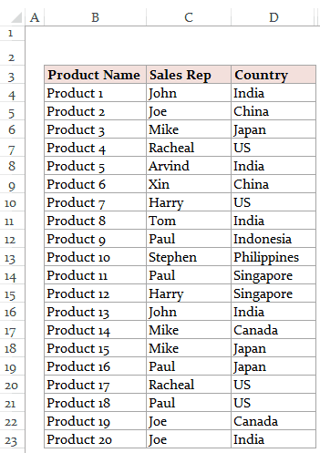
USEFUL TIP: It is almost always a good idea to convert your data into an Excel Table. You can do this by selecting any cell in the dataset and using the keyboard shortcut Control + T.
Step 1 – Getting a unique list of items
- Select all the Countries and paste it into a new worksheet.
- Select the country list –> Go to Data –> Remove Duplicates.

- In the Remove Duplicates dialogue box, select the column in which you have the list and click Ok. This will remove duplicates and give you a unique list as shown below:

- One additional step is to create a named range for this unique list. To do this:
- Go to Formula Tab –> Define Name
- In Define Name Dialogue Box:
- Name: CountryList
- Scope: Workbook
- Refers to: =UniqueList!$A$2:$A$9 (I have the list in a separate tab named UniqueList in A2:A9. You can refer to wherever your unique list resides)

NOTE: If you use ‘Remove Duplicates’ method and you expand your data to add more records and new countries, you will have to repeat this step again. Alternately, you can also you a formula to make this process dynamic.
See Also: How to use a formula to get a list of Unique items.
Step 2 – Creating The Dynamic Excel Filter Search Box
For this technique to work, we would need to create a ‘Search Box’ and link it to a cell.
We can use the Combo Box in Excel to create this search box filter. This way, whenever you enter anything in the Combo Box, it would also be reflected in a cell in real-time (as shown below).

Here are the steps to do this:
- Go to Developer Tab –> Controls –> Insert –> ActiveX Controls –> Combo Box (ActiveX Controls).
- If you do not have the Developer Tab visible, here are the steps to enable it.

- Click anywhere on the worksheet. It will insert the Combo Box.

- Right-click on Combo Box and select Properties.
- In Properties window, make the following changes:
- Linked Cell: K2 (you can choose any cell where you want it to show the input values. We will be using this cell in setting the data).
- ListFillRange: CountryList (this is the named range we created in Step 1. This would show all the countries in the drop down).
- MatchEntry: 2-fmMatchEntryNone (this ensures that a word is not automatically completed as you type)

- With the Combo Box selected, Go to Developer Tab –> Controls –> Click on Design Mode (this gets you out of design mode, and now you can type anything in the Combo Box. Now, whatever you type would be reflected in cell K2 in real time)
Step 3 – Setting the Data
Finally, we link everything by helper columns. I use three helper columns here to filter the data.
Helper Column 1: Enter the serial number for all the records (20 in this case). You can use ROWS() formula to do this.
Helper Column 2: In helper column 2, we check whether the text entered in the search box matches the text in the cells in the country column.
This can be done using a combination of IF, ISNUMBER and SEARCH functions.
Here is the formula:
=IF(ISNUMBER(SEARCH($K$2,D4)),E4,"")
This formula will search for the content in the search box (which is linked to cell K2) in the cell that has the country name.
If there is a match, this formula returns the row number, else it returns a blank. For example, if the Combo Box has the value ‘US’, all the records with country as ‘US’ would have the row number, and rest all would be blank (“”)
Helper Column 3: In helper column 3, we need to get all the row numbers from Helper Column 2 stacked together. To do this, we can use a combination if IFERROR and SMALL formulas. Here is the formula:
=IFERROR(SMALL($F$4:$F$23,E4),"")
This formula stacks all the matching row numbers together. For example, if the Combo Box has the value US, all the row numbers with ‘US’ in it get stacked together.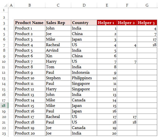
Now when we have the row numbers stacked together, we just need to extract the data in these row number. This can be done easily using the index formula (insert this formula in where you want to extract the data. Copy it in the top-left cell where you want the data extracted, and then drag it down and to the right).
=IFERROR(INDEX($B$4:$D$23,$G4,COLUMNS($I$3:I3)),"")
This formula has 2 parts:
INDEX – This extracts the data based on the row number.
IFERROR – This returns blank when there is no data.
Here is a snapshot of what you finally get:
The Combo Box is a drop down as well as a search box. You can hide the original data and helper columns to show only the filtered records. You can also have the raw data and helper columns in some other sheet and create this dynamic excel filter in another worksheet.
Download the Dynamic Excel Filter Example File

Get Creative! Try Some Variations
You can try and customize it to your requirements. You may want to create multiple excel filters instead of one. For example, you may want to filter records where Sales Rep is Mike and Country is Japan. This can be done exactly following the same steps with some modification in the formula in helper columns.
Another variation could be to filter data that starts with the characters that you enter in the combo Box. For example, when you enter ‘I’, you may want to extract countries starting with I (as compared with the current construct where it would also give you Singapore and Philippines as it contains the alphabet I).
As always, most of my articles are inspired by the questions/responses of my readers. I would love to get your feedback and learn from you. Leave your thoughts in the comments section.
Note: In case you’re using Office 365, you can use the FILTER function to quickly filter the data as you type. It’s easier than the method shown in this tutorial.
You May Also Like the Following Excel Tutorials:
- Highlight Matching Data Using Conditional Formatting – Dynamic Search.
- Create a Search Suggestion Drop Down List in Excel.
- Using Advanced Filter in Excel.
- How to Extract a Substring in Excel (Using TEXT Formulas).
- Creating a Drop Down Filter to Extract Data Based on Selection.
- How to Filter Cells with Bold Font Formatting in Excel.
- Highlight Rows Based on a Cell Value in Excel.
- VBA AutoFilter in Excel: Syntax, Criteria, and Examples

Hello Sumit, thank you for your wonderful and very helpful tutorial. Question, I have certain questions that are highlighted but when they are extracted they’re no longer highlighted, how can I keep the questions in the same style?
thank you for your amazing knowledge.
हिन्दी में बताइए
This is brilliant! Thanks for the sharing! Very useful!
This was great Sumit! Very helpful. I ran into one problem and was wondering if you knew a quick fix. If it was mentioned already in the comments, please let me know and I’ll go find it. In my list, I have terms such as NBC, MSNBC, CNBC, etc. When I do the drop down selection for MSNBC, I only get results for MSNBC (which is good!) However when I do the drop down selection for NBC, I get results for anything related to NBC (NBC, MSNBC, CNBC, NBCSN, etc). Is there a way for me to isolate just NBC? Thanks
~Brian
Hi there, can I embed this feature on my website?
Great article Sumit. Thanks for sharing 🙂
I’ve just discovered a pretty good video where the search filter works dynamicaly by hiding the rows. Looks very nice and useful. Moreover, there is a download link below the video, so you can try it immediately.
https://www.youtube.com/watch?v=iZ933-tU6Yw
Maybe you will find there some new ideas..
thanks yu, you are really helping me a lot.. keep up your good work. god of excel 🙂
Hi… Thanx for the great post…it was really helpful !!!
I want to do something similar, but rather than filtering on the column i want to filter by row.
i.e. You are showing a row if it the cell has the particular value, I want to show the columns if the cell in it has the particular value. I am able to write formulas for populating the helper columns.
But am stuck with the last one to populate the final set.
Can you please help with this?
Thank you for the video. What if I want to extract any data that I type in the combo box, what would the formula be? Thanks.
Is there a way to auto fill repetitive data like name and address?
Hello Robert.. have a look at this tutorial: http://trumpexcel.com/2014/05/let-excel-complete-abbreviations-for-you/
Thanks Sumit for the reply and pointing me to the right topic. I will check out the link.
I did check the link but it does not suit what I was looking for. This is the actual scenario what I am looking for maybe you can point me to the right topic. We have to input name of companies to Excel based on the Invoice issued, the name would occur several times. Together with the name there is assigned Tax Identification Number that would be inputted beside the company name. I would appreciate any help.
Fantastic demo, well written. I’m a little confused why you need to create a unique table, why not dump all your raw data on one sheet (in my case, priority, alarm, information, support team) and have another sheet do the search and display the relevant rows below ? This would (I think) be more universal and help more people. Just a thought, not by any means a criticism.
Thanks for sharing Miles.. Unique list is created for the drop down, so that there are no repetitions in that. If that’s not needed, that you can do away with the unique list step
Hello,
If I have dates in mm/dd/year (or some equivalent) how can I use the dynamic filter to search by month or year whilst keeping the date format?
Unfortunately even if the dates are formated to say the respective month it only searches in based off of what is in the formula box.
I look forward to your response.
Hi Sumit, thanks for this. It’s a great tutorial. I have a couple of further issues I’m hoping you can help me with. In my filtered results any cells that were left blank in the raw data now have a 0 (zero) in them. Is there a way to show the cells as blank in the filtered results? Also, some of the filtered cells contain hyperlinks. These are “live” in the raw data (if you click them they open the relevant page in your browser), but they are not live in the filtered data. Is there a way to make them live in the filtered data? Thanks for any help you can give!
hello, thanks for your post. but i noticed the first formula doesn’t work for me
HOW DO I SELECT ONLY ITEMS THAT START WITH THE CHARACTER I WANT. IF I ENTER “PH” I WANT TO RETRIEVE PHILLIP NOT ALPHOSO…YOU MENTION TWEEKING THE HELP BUT I’M NOT SURE HOW..
Hello. Thank you for the superb post. You saved me big time. But there’s a problem. The search box also filter the words that contain the words I search. For example, I search for “AN” and the rows with “CHANH” also appear. How can I set it so that only the exact word is filtered?
Hello Minh. You can do that by replacing the formula in Helper 2 with the following: =IF(AND(ISNUMBER(SEARCH($K$2,D4)),LEN(D4)=LEN($K$2)),E4,””)
Simply put this formula in F4 and copy for all the cells in that column.
Hi Sumit, Can you show how to add two filters, Country and Product? How can that be done?
Hello.. Have a look at this file: https://www.dropbox.com/s/junqiduvcu929im/Dynamic-Excel-Filter%20-%202%20conditions.xlsx?dl=0
Hello, Is it possible to take the range of the ‘Filtered Data’ section from one sheet to another?
If I copy the formula over and add the sheet name before the cell I can see all the current values, but it doesn’t appear to be dynamic and update like the information does on the original sheet.
any help is appreciated.
Hello JP.. You can get the filtered data in another sheet as well. Instead to adding the sheet name manually, I would suggest you reconstruct it from scratch (as shown in the tutorial). That way Excel will take care of the cell referencing and naming itself
Hi Sumit
This is a brilliant method for making a searchable staff telephone list. However, some of my cells in the range are blank, where there is either no extension or mobile, and they are showing in the search result table as 0. I have tried, without success, to add an if statement to weed these out and show them as blank cells. Is there a way to do this without causing the formula =IFERROR(INDEX($B$4:$D$23,$G4,COLUMNS($I$3:I3)),””) to throw up an error?
Hello Dawn.. Would be great if you could paste a screen shot of the data, or send me the data via email. I just want to make sure I give you the formula that suits your data. It can be done by tweaking existing formulas used in the template
Hi Sumit,
Thanks for sharing!
I am currently putting the dynamic filter and its data on a different worksheet. May I know if it is possible to also have a filter option to display “All the data”.
If I would like to have the option to choose “All Countries” from your example, how would I be able to do it?
Hello Jo. You can do that by changing the formula in Helper Column2. Here is a template that gives the option to select all countries – https://www.dropbox.com/s/sczdl872t74say2/Dynamic-Excel-Filter_All%20Countries.xlsx?dl=0
When the combo box is empty it shows the entire result(s). Is there a way when the combo box is empty the results are blank?
Hello Rob.. change the formula in Helper Column 2 with the following formula: =IF(AND($K$2″”,ISNUMBER(SEARCH($K$2,D4))),E4,””)
Now when the combo box is empty, it will show no results
Hi Sumit, is it possible to search 2 items at the same time for example: all the US and the Canada ?
Hello Elyse..Yes you can have filter on multiple conditions. The formula needs to be changed to make it OR instead of AND. Have a look at this file where you can filter based on two countries https://www.dropbox.com/s/q49v1qhuozxnrq9/Dynamic-Excel-Filter%20-%202%20conditions%20Same%20Country.xlsx?dl=0
Hi Sumit – this is awesome! Just wondering if you’re able to help me out a little bit more?
I’m trying to do a version of this where the data is output to a second sheet (saves me from hiding & unhiding cells all the time).
I’ve managed to output the data to a sheet named UI (user interface) but now the search filter isn’t working. It’s probably something to do with how I’ve written the Formula’s, but I can’t figure it out.
I’ve attached screenshots showing the sheets and the formula’s being used. Any help would be much appreciated!
Cheers,
Jen
Hello Jen.. Can you share the file (may be a dropbox or onedrive link). I can’t see snapshots here
This is super awesome ! One quick question: can we highlight the keywords in some color in the database as we type and it hits the match. Please let me know
Thanks for commenting Shameek.. Here is a tutorial to highlight the matching rows as you type in a search box – http://trumpexcel.com/2013/07/search-in-excel-conditional-formatting/
I checked this one before, not working for me. I already have a dynamic filter using the formula what’s it’s shown here, now i want to color code only texts while typing using the same dynamic filter .. I have used 3 helper and the formula is the same what’s shown in this. Also I have created a front end where showing the search results but the color coding is not working. Don’t know why.
Sir, Thank you so much for the tutorial, you save my family’s business.
I do have a bit of question. Instead of country name like Japan, India, Singapore, I have a “group id” like 001, 01, 240, 24, 924. And I did >Define Name and all. But once I start using the combo box, “24”, the items of other group like 240 and 924 would come along.
I guess it has something to do with The helper 2 column “=IF(ISNUMBER(SEARCH($K$2,D4)),E4,””)”
Could you please help me to search the result of the exact value? Thank you so much !
Hello Seebear.. You can do that by changing the formula in Helper Column 2 to =IF($K$2=D4,E4,””)
hi i m sumeet , sir i want to know that can i edit the data selected from the drop down list on real time , for eg. i have selected sumeet as my name from the drop down list & i want to add singh as my surname after my name on real time basis
This was so helpful. Thank you. I had been banging my head all week trying to do this on my own.
Only issue I encountered is after selecting the item from the Combo list, sometimes the selection just disappears – i.e. the combolist seems to just clear itself. Not sure what is going on there. Do you have any idea what could be causing this please?
can we add 3 or 4 columns in data and shown in filtered data
Hello Sumit, thanks a lot very helpful site!! I have been trying for days now without getting any solution. Is there a way to edit the filtered values? for example I type Japan. Then once I have the filtered results I go and change/update the Sales Rep name?
hi. if I have 6 columns, then i will be having 6 helper?? pls answer. thanks
hi Sir,
i have tried it on my datasheet using the same formulas but it seen like i cant filter the information what i want.
can you able to see what wrongs with my formula?
thank you in adance
Hi,
As i mentioned in the comments below. I’ve got a pretty large dataset for which this solution really struggles. and takes good few seconds to filter through data. I’ve just read about INDEX MATCH formula – so was wondering if this type of dynamic search could be achieved using INDEX MATCH formula, which should be most probably quicker than the INDEX you have used here. Please advise.
Thank you
p.s. more about INDEX MATCH benefits: http://www.mbaexcel.com/excel/why-index-match-is-better-than-vlookup/
Hello Sumit,
Thank you so much for uploading this video. Is there any way to show the search result blank if there is no data in the combobox ?
Hello Siddhartha.. Thanks for dropping by and commenting. You can do this by changing the formula in 2nd helper column to: =IF(LEN($K$2)=0,””,IF(ISNUMBER(SEARCH($K$2,D4)),E4,””))
Paste this formula in F4 and drag it down.
Hi Sumit,
Thanks for your sharing, if the data table have a blank in somewhere cell, it doesn’t count this row, any formula can solve it?
Keep going, i am a fan of this website.. Gaurav Negi
Thanks for commenting Gaurav,, Glad you like the tutorials here 🙂
Hi Sambit,
Regarding the variations: I’m wondering if it’s possible to have more than two conditions/filters? I can’t seem to figure out the correct formula.
Thanks!
Hello Anna, Have a look at this file. I have created the filter for 2 conditions – https://www.dropbox.com/s/junqiduvcu929im/Dynamic-Excel-Filter%20-%202%20conditions.xlsx?dl=0
Hi again Sumit,
I’ve downloaded that version and applied the formula to my spreadsheet. It works perfectly for two conditions, but I can’t figure it out for more than two. Is this possible? Sorry if this isn’t clear!
have a look at this – I have used 3 conditions here – https://www.dropbox.com/s/sumo1l3b37nc1jm/Dynamic-Excel-Filter%20-%203%20conditions.xlsx?dl=0
You need to modify the formula in second helper column to check for all 3 conditions
AMAZING! Thank you so much for your quick response. Is there a maximum condition limit, or can you use as many conditions as you like? Thank you again!
Glad it helped.. The number of conditions depends on the data, In this case, we have 4 columns of data, so there could be 4 conditions. AND formula can handle a maximum of up to 30 conditions
I added another condition and it worked. Thank you so much again for your help, it’s much appreciated!
Hi Sumit, would you please share the formula to include up to 30 conditions again please? I can’t seem to be able to access the file via the dropbox link above. It would help very much!
Thank you!!
Gr8, but Combo Box 2 is drop down list is carrying sales rep data, though in case I type any name of product category, it’s ok.
Nice,works well, but unusable with big tables, takes 5 min to filter a 12k row table on a Quad Core i5 with 4G RAM. I am aware this is not the intended use, just want to inform others who want to give it a try 🙂
Hi.
I’m in the same situation as posted above. I’ve got a file of 15 000 rows and the list is constantly growing. I’ve tried the formula with helper columns and all works great, apart that it takes around 1-3 seconds to generate a list from my query. Also the way i made a formula is to output the data to another sheet as a summary instead of seeing all raw data, so it looks really need. I’ve also tried the same solution with the 1 000 entries and that returns data as i type. I’ve got i5 6 GB laptop and it really struggles with the large database (15k rows). Is there another way of making the same dynamic search that wouldn’t put so much pressure on processor and would return data as i type?
Also big thanks for trumpexel for such a great solution.
Hi there 🙂 Suppose I have hyperlinks instead of text data in the specific columns, how do I retain the hyperlink and not extract the data as text after the search
Have a look at this technique – http://trumpexcel.com/2014/03/create-dynamic-hyperlinks-in-excel/
You would need to club the 2 to get dynamic filter that retain hyperlinks
ahh ok thanks for the prompt reply!
Club the two? I have web links in the “Sales Rep” Column. How do I get it to retain the hyperlink after it has been searched? This has been very helpful so far. Thanks!
I have a huge data approx. 50,000 rows and i want to filter it with search box as i start typing in the search box the data starts to filtering but i am failed to do it.
Your example is too good but I don’t want to use “INDEX” formula.
Please help me out.
Hi.
I’m in the same situation. I’ve got a file of 15 000 rows and the list is constantly growing. I’ve tried the formula with helper columns and all works great, apart that it takes around 1-3 seconds to generate a list from my query. Also the way i made a formula is to output the data to another sheet as a summary instead of seeing all raw data, so it looks really need. I’ve also tried the same solution with the 1 000 entries and that returns data as i type. I’ve got i5 6 GB laptop and it really struggles with the large database (15k rows). Is there another way of making the same dynamic search that wouldn’t put so much pressure on processor and would return data as i type?
Also big thanks for trumpexel for such a great solution.
Hi Sumit,
You wrote this “You can try and customize it to your requirements. You may want to create 2 filter instead of one. For example, you may want to filter records where Sales Rep is Mike and Country is Japan. This can be done exactly following the same steps with some modification in the formula in helper columns.”
Could you please tell me what changes to make in helper columns to make 2 filters work?
Thanks a lot!
Kindly let me know.
Best Regards,
Karthik
Have a look at this – https://www.dropbox.com/s/junqiduvcu929im/Dynamic-Excel-Filter%20-%202%20conditions.xlsx?dl=0
I have added another filter and changed the formula in the helper columns
Thanks Sumit, i tried that, but it gives me a message “we found one or more circular references that might cause your formulas to calculate incorrectly”. is there something I can look out for to resolve this problem?
Hey Karthik.. Are you talking about the file I shared, or something you created? The file I have shared works fine on my system. I checked and there are no circular reference errors. If it’s a file you have created, kindly share with me and I can have a look
You can try and customize it to your requirements. You may want to create 2 filter instead of one. For example, you may want to filter records where Sales Rep is Mike and Country is Japan. This can be done exactly following the same steps with some modification in the formula in helper columns.
Sumit, Could you please tell me how to use 2 filters, i.e. what changes to make in the helper columns?
Thanks
hi, this is very useful for my task. But I need one that can hyperlink also. Does this dynamic filter can be linked to other file such as pdf file? For example, if I click product 1 in the filtered table, I expect that it will open another file consists of product 1 data. Is it possible? Thanks
It can be done if you are looking to hyperlink within the same workbook. Have a look at this – http://trumpexcel.com/2014/03/create-dynamic-hyperlinks-in-excel/
I guess I can’t link it to other file like .doc? only to data in the same workbook
What if I want to Hyperlink to a website?
Yes . I have a database where there are 50 columns and each column has
10000 rows , with new entries being added each day . I want 50 dynamic
filters on each column so that i dont have to scroll the page for
applying filters on each column . As i want to filter data with
combination of any number of columns , i was looking for multiple
dynamic filter . Basically i want to use normal filters to filter data ,
with the exception that i can place the combobox as per my convenience
. Also if you can tell any technique wherein when I type the data in
dynamic filter it gives a google type search dropdown also , it will be most
helpful . Thanks
this was really helpful .. can anyone tell how to make more than one dynamic filter in this
Glad you liked it.. What do you mean by more than one filter. Are you looking for more than one criteria?
Great Bansal sahab
Thanks for commenting.. Glad you liked it 🙂
hi Sumit,
two days back only I came across your site and just looking through..it makes me wonder!!
Keep on keeping On.
Amal
Hello Amal.. Welcome to Trump Excel and Thanks for commenting.. I am really glad you found the website useful 🙂
Hey, great idea and implementation. I might use it at school to teach the kids a few tricks. Can all of this be done with a text field instead of drop-box?
Thanks for commenting and glad you liked it 🙂 I am afraid I not aware of any way to do this without combo-box. The benefit for combo-box is that it makes the data entry dynamic, which instantly gives you results.
This is worked perfect! I have a table with 830 rows that displays totals at the bottom of each column; and each filter option will result in about 200 rows. The problem that I have now is that I have to scroll all the way down to row 831 in order to see the totals. This document will also be printed by end users and I would like to avoid the extra blank papers. Any suggestions will be highly appreciated.
Hi Michelle.. you can try this formula:
=IF(AND(G3″”,G4=””),SUM($G$4:G4),IFERROR(INDEX($B$4:$D$23,$G4,COLUMNS($I$3:J3)),””))
I have made it based on the data set I have provided in the download file (assuming Column C has numbers)
Very cool
Thanks Buddy.. Glad you liked it 🙂
It is really helpful
Thanks for the comment Uday.. Glad you liked it 🙂
Thanks for commenting Uday..Glad you liked it 🙂
Thanks alot for this great video , it helped me alot , God bless you
Hey, I did it without Helper and Array. For intermediate level, it’s bit complex 🙂
{=IFERROR(INDEX($B$2:$D$21,SMALL(IF(ISNUMBER(SEARCH($U$1,$D$2:$D$21)),ROW($D$2:$D$21)-1,””),ROW()-4),COLUMNS($L$4:L4)),””)}
Hello Deepak.. Thanks for commenting and sharing the formula 🙂
Hi Deepak, can you maybe brake your formula down into smaller segments so i can understand what and how you did it. Also i’m trying to find a way to work with 15k lines of dataset which Trumpexel is not really coping well with as it takes 3-4 seconds to give the results on i5 6GB RAM processor. So i wonder if your formula would be any quicker as it wouldn’t need helper colums. please advise.
Thank you
dragging the array formula till 15k row will make the excel sheet slow..
Hello Deepak, i’m really interested in seeing the rest of your formula here, for some reason it’s cutting it off after ROW($D$2:$D$21)-1,””),
I know it was a long time ago, but if you could possibly reply with the rest of the formula i would really appreciate it!
Nevermind, it appeared when I opened in a different browser, thank you!
Thanks Randy, you know it takes time to understand my own complex formula 🙂 lol …
Hey Deepak Could u share your excel sheet. Your formula is little bir confusing
Its difficult to find the excel file, what i have done is – i have incorporated all the helper formula in one formula..so it became big.
Sure but i can’t upload the excel file here, can you please share your Email Id so that i can send it to you.
b.alperkaya@gmail.com
Sent
Hi Deepak, would you be able to send me a copy of the corresponding excel file please to help understand your formula a bit better? Thanks in advance!
Pls share your email so that I can send you the file.
Do you know how can I multiple excel filters with your formula?
Thank you,
Really it’s great…….
Thanks for commenting Sambit.. Glad you liked it 🙂
Hello Bansal,
i’m new on the forum. i looking for a way to do exactly what you describ in this topic.
from the bebening, it works well. but when it come to apply the formulla, it became confused for me. the formula doesn’t work on my side.
it come with mistake from the helper column 2 :=IF(ISNUMBER(SEARCH($K$2,D4)),E4,””)
can you help me please.
will be gratfull
Isaac