

Excel Filter is one of the most used functionalities when you work with data. In this blog post, I will show you how to create a Dynamic Excel Filter Search Box, such that it filters the data based on what you type in the search box.
Something as shown below:

There is a dual functionality to this – you can select a country’s name from the drop-down list, or you can manually enter the data in the search box, and it will show you all the matching records. For example, when you type “I” it gives you all the country names with the alphabet I in it.
Download Example File and Follow Along
Watch Video – Creating a Dynamic Excel Filter Search Box
Creating a Dynamic Excel Filter Search Box
This Dynamic Excel filter can be created in 3 steps:
- Getting a unique list of items (countries in this case). This would be used in creating the drop down.
- Creating the search box. Here I have used a Combo Box (ActiveX Control).
- Setting the Data. Here I would use three helper columns with formulas to extract the matching data.
Here is how the raw data looks:
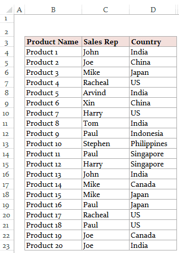
USEFUL TIP: It is almost always a good idea to convert your data into an Excel Table. You can do this by selecting any cell in the dataset and using the keyboard shortcut Control + T.
Step 1 – Getting a unique list of items
- Select all the Countries and paste it into a new worksheet.
- Select the country list –> Go to Data –> Remove Duplicates.

- In the Remove Duplicates dialogue box, select the column in which you have the list and click Ok. This will remove duplicates and give you a unique list as shown below:

- One additional step is to create a named range for this unique list. To do this:
- Go to Formula Tab –> Define Name
- In Define Name Dialogue Box:
- Name: CountryList
- Scope: Workbook
- Refers to: =UniqueList!$A$2:$A$9 (I have the list in a separate tab named UniqueList in A2:A9. You can refer to wherever your unique list resides)

NOTE: If you use ‘Remove Duplicates’ method and you expand your data to add more records and new countries, you will have to repeat this step again. Alternately, you can also you a formula to make this process dynamic.
See Also: How to use a formula to get a list of Unique items.
Step 2 – Creating The Dynamic Excel Filter Search Box
For this technique to work, we would need to create a ‘Search Box’ and link it to a cell.
We can use the Combo Box in Excel to create this search box filter. This way, whenever you enter anything in the Combo Box, it would also be reflected in a cell in real-time (as shown below).

Here are the steps to do this:
- Go to Developer Tab –> Controls –> Insert –> ActiveX Controls –> Combo Box (ActiveX Controls).
- If you do not have the Developer Tab visible, here are the steps to enable it.

- Click anywhere on the worksheet. It will insert the Combo Box.

- Right-click on Combo Box and select Properties.
- In Properties window, make the following changes:
- Linked Cell: K2 (you can choose any cell where you want it to show the input values. We will be using this cell in setting the data).
- ListFillRange: CountryList (this is the named range we created in Step 1. This would show all the countries in the drop down).
- MatchEntry: 2-fmMatchEntryNone (this ensures that a word is not automatically completed as you type)

- With the Combo Box selected, Go to Developer Tab –> Controls –> Click on Design Mode (this gets you out of design mode, and now you can type anything in the Combo Box. Now, whatever you type would be reflected in cell K2 in real time)
Step 3 – Setting the Data
Finally, we link everything by helper columns. I use three helper columns here to filter the data.
Helper Column 1: Enter the serial number for all the records (20 in this case). You can use ROWS() formula to do this.
Helper Column 2: In helper column 2, we check whether the text entered in the search box matches the text in the cells in the country column.
This can be done using a combination of IF, ISNUMBER and SEARCH functions.
Here is the formula:
=IF(ISNUMBER(SEARCH($K$2,D4)),E4,"")
This formula will search for the content in the search box (which is linked to cell K2) in the cell that has the country name.
If there is a match, this formula returns the row number, else it returns a blank. For example, if the Combo Box has the value ‘US’, all the records with country as ‘US’ would have the row number, and rest all would be blank (“”)
Helper Column 3: In helper column 3, we need to get all the row numbers from Helper Column 2 stacked together. To do this, we can use a combination if IFERROR and SMALL formulas. Here is the formula:
=IFERROR(SMALL($F$4:$F$23,E4),"")
This formula stacks all the matching row numbers together. For example, if the Combo Box has the value US, all the row numbers with ‘US’ in it get stacked together.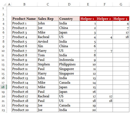
Now when we have the row numbers stacked together, we just need to extract the data in these row number. This can be done easily using the index formula (insert this formula in where you want to extract the data. Copy it in the top-left cell where you want the data extracted, and then drag it down and to the right).
=IFERROR(INDEX($B$4:$D$23,$G4,COLUMNS($I$3:I3)),"")
This formula has 2 parts:
INDEX – This extracts the data based on the row number.
IFERROR – This returns blank when there is no data.
Here is a snapshot of what you finally get:
The Combo Box is a drop down as well as a search box. You can hide the original data and helper columns to show only the filtered records. You can also have the raw data and helper columns in some other sheet and create this dynamic excel filter in another worksheet.
Download the Dynamic Excel Filter Example File

Get Creative! Try Some Variations
You can try and customize it to your requirements. You may want to create multiple excel filters instead of one. For example, you may want to filter records where Sales Rep is Mike and Country is Japan. This can be done exactly following the same steps with some modification in the formula in helper columns.
Another variation could be to filter data that starts with the characters that you enter in the combo Box. For example, when you enter ‘I’, you may want to extract countries starting with I (as compared with the current construct where it would also give you Singapore and Philippines as it contains the alphabet I).
As always, most of my articles are inspired by the questions/responses of my readers. I would love to get your feedback and learn from you. Leave your thoughts in the comments section.
Note: In case you’re using Office 365, you can use the FILTER function to quickly filter the data as you type. It’s easier than the method shown in this tutorial.
You May Also Like the Following Excel Tutorials:
- Highlight Matching Data Using Conditional Formatting – Dynamic Search.
- Create a Search Suggestion Drop Down List in Excel.
- Using Advanced Filter in Excel.
- How to Extract a Substring in Excel (Using TEXT Formulas).
- Creating a Drop Down Filter to Extract Data Based on Selection.
- How to Filter Cells with Bold Font Formatting in Excel.
- Highlight Rows Based on a Cell Value in Excel.
- VBA AutoFilter in Excel: Syntax, Criteria, and Examples

Great article that I have immediately put to use! How would I have the cursor default to being inside the combo box when the workbook is opened? Thanks
This is a brilliant tutorial with a very effective final result. Thanks for laying this out. I’ll be using this over and over again, I’m sure. FANTASTIC!
Excellent Video.
I was thinking how it would be possible to apply this advance filter and then have the option to input data into the filtered products.
Example I filter for India, it bring up 4 result and then I want to input data to the results. More like i’m filtering the actual entire row of the result?
You response will be greatly appreciated.
hi, I have been using this dynamic filter system for years and it works brilliantly!!!.
One thing that was not needed was the drop down choice to be filtered, but
recently I have re-used this idea and again it works perfectly but….. this time the drop down filter to choose just a letter and it filter the results would be wonderful, but it just doesn’t work. I have downloaded the excel file and have copied everything to the letter but it just chooses the full name of the selection. Can anyone help.
Hi Sumit,
I’ve found your video extremely useful, but like a lot of others I’m struggling to apply your formula to multiple searches/filters/conditions. I’ve seen you’ve shared a dropbox link for this solution but they have expired. Is it possible to please create another link or to comment in an example of this formula – this would be much appriciated.
Many thanks,
Jack
Hi There,
It really helped me do the search bar and it works fine,
however, my data is huge and it takes lot of time to get the output and it keeps calculating.
Kindly suggest on the concern.
You are really good
How do I create this for multiple excel filters? Let’s say, I want to put in a second filter.
Hey Bradley – did you figure this out? I am trying to do the same
Hey, no I didn’t figure it out; hoping someone would lend a hand
It says above it can be done ‘exactly following the same steps with some modification in the formula in helper columns.’
Can anyone help??
I did get this to work with multiple filters. Use the search for multiple selections (Column Helper 2 – apply for each sort field) to come up with the data columns, and then use a separate column to call out where the various columns all have the same data. I did three helper columns with a sort of “if Helper 1 = Helper 2 = Helper 3 then show value in Helper 1”. Then I did the sort in Helper 3 off of the new column and it worked.
I hope that makes sense…
how if searching in multiple sheets
=IFERROR(INDEX(‘DAY1′!$B$6:$O$55,’DAY1’!$S6,COLUMNS($B$10:B10)),””)
day 1 = 1 sheet up to 31 sheet
I like your post it is very informational. Kindly also make post to use this search filter in vba form
Another variation could be to filter data that starts with the characters that you enter in the combo Box. For example, when you enter ‘I’, you may want to extract countries starting with I (as compared with the current construct where it would also give you Singapore and Philippines as it contains the alphabet I).
I would love to know will I do the above statement. and btw thankyou for the video it really helo me a lot. the only thing that i need to do is the statment above.
I hope you will answer this
So effective… Thank you so much !
One improvement would by to allow us to search for multiple words.
What if i would like to have the entire spreadsheet to be filtered to only extract data with everything that contains “la” or “east”. This formula only allows for data from a specific column. How can this be accomplished?
hi
please I have different sheet each one of them have the same think just different company name. i want to have as in this exemple but result in an other sheet and also the data coming from different sheet
thanks
I know this is old, but I know too that a lot of people still uses this topic. It’s so useful! But I’d like to know if there is any way to make the search box better, I mean, searching Products, Sales Rep and Countries. Not ONLY contries. Thanks!
hi
first, thank you for this excellent work :
I need, please your help if you can.
I want to know I want to create this filter first with more than 15 worksheets and each one having the same column and rows information.
I want to create a comparison tool, as if, I enter for example item number or name will give me a grill with what I need in a unique worksheet as an output.
Here is what I have :
1- 15 worksheets: each worksheet, it’s for a specific company, each sheet has the same thing: ex:
item name, prices, capacity, our prices, margin, etc..
2- I want to make a search ( as you did in the box you create ) when I search for example by name:
*** My result expected: will give a table with the less price first and which company is associated with.
3- is it possible to do with excel, if not can you guide me please, which program I can need to use is it a database +VB or what exactly, please.
Thanks a lot.
sorry,its doesn’t work over 313 rows,what i should do?
Can I make it show no result until/unless I type something in the search box?
Can a search box be created in a second sheet using the data from sheet1?
I have about 2500 line items (Inventory) and 7 header columns. I currently use Conditional formatting but the problem is scrolling down the page to see what is highlighted.
Yes, you can.
Make these “helpers” in the sheet where all the data is.
Then, in the secondary sheet, make a table with Filtered Data.
=IFERROR(INDEX((dataSheet!$B$4:$D$23000);(dataSheet!$G4);COLUMNS(showSheet!$A$4:A4));””)
Is there a way to then be able to sort through this list? When I sort, some blank rows appear
Sort Z>A not A>Z
I need to use a dynamic filter text for online usage, with a shared website in my company. How can I use ActiveX Dynamic filter this way?
How can I do this if I don’t have a designer license?
Would it be possible to set up 2 columns, where the first column has multiple looks for “this” AND “that”, and the second column has fields that looks for “this” OR “that”, and return the results in the same column?
Very nice
Extremly super admin.. i appreciate it a lot. thank you so much.
can you do the filter without using helper columns? i mean, filtering the data table?
How do you make it so that hyperlink would stay intact in your search results?
how can i provide security for this file.i mean we have a cleint list.the flle shall be available for everyone in office.i can protect workbook with a password. but search bar also getting password protection. what can i do
hi, could we make this filter but with additional conditions instead of just 1 condition?
Hello,
I have successfully completed this; however, one of my columns with information the populates contains hyperlinks to documents on the computer. Right now these hyperlinks are only showing up as text. I would like the link to be retained when it appears in the search results, can you help with this?
Hi Sumit, can you tell me how can I customize the text search to show only the specific text I am looking for? Current formulas return any text that contains what was entered in the text box.
Thank you for your help,
Enna
I’m also having this problem. Any help would be appreciated!
hi…
if there are multiple rows then what should be done in helper coloumns…. do i setup the helper 4 row and which formula i have to enter…
please do needful help
This works great for my needs! I would like to hide the dynamic list while the search box is empty and only show the results. Is there a way to do this?
I like the idea (and I’m guessing this is pretty old) but this is the most round about way I’ve ever seen to accomplish this. What you really want is to simply work the autofilters via the combobox’s change event. if you need to view your filtered data on a separate sheet then simply copy the filtered range to it. No need for helper columns or vlookup/index formula’s either. You could also use a dynamic range in VBA and forget about the static named range altogether.
Just my 2cents…
Hi SM177y
can you please elaborate on this?
I think you are referring to manage large number of data rows
I have around 10K rows and the original equation in this post is little slow.
how can i improve this?
Hello. This is a great tutorial and is just what I was looking for. However, I’m stuck on Helper 3. In the YouTube video you mention something about adding ROWS. I can’t see the formula because the video is a little blurry. In the instructions above, there is no mention of rows. When I follow the instructions above, I’m not getting my numbers stacked in Helper 3.
Hello.. The ROWS function is used in Helper Column 1. The formula used in cell E4 is =ROWS($B$4:B4) and then copied for all the remaining cells in the column. You can also download the example file and see the exact formula in it.
Hi Sumit, just to check can we select two filters like maybe one box for both country and name or two boxes , one for country and one for name. How would the excel sheet formula be like? Thanks in advance
I am still a relative novice with excel, so forgive me if my question seems silly. I was fine until I got to creating the index. When I try to drag the formula down and to the right, it changes the formula in the other boxes in such a way that the search doesn’t bring up the proper information. Basically the formula changes by shifting the area of information either down a row or one column to the right. Is there a way to prevent it from changing anything other than what is necessary for accuracy so I don’t have to manually go in and fix it?
Straight forward with clear explanations! Sambit you are an excellent trainer 🙂
This is brilliant, thanks a lot for posting it!
too good, but this formula only on 20 cell i need it on 2k cell please help me!
i need this formula, but its work only with 20 cell in need it till 2k cells. please help me?
Following this guide, to use it on a larger data set, you would only need to redefine the named range to include however many rows you need….But if you read my other comment and do a little Googling, you’ll find much easier, faster, and more efficient ways to accomplish this that aren’t bound to any static range.
Is there a way how I could add more than 1 dynamic filter in a sheet? Let’s say first I sorted all which were for India, and then via second one I need to sort only Sales Rep John within India. Thanks in advance. Emil
Many thanks for this. I was able to follow your very clear explanations. Works remarkably well. I’d like to add a button to clear the search field. I wonder if you would mind sharing any suggestions?
Thanks a lot
Hi Sumit,
I would like to make dynamic books title list with the help of this formula, can you suggest further options to me e.g. – once a user will get the data after applying drop down option after this can he directly email the outcome to clients or save the outcome in PDF
email – varunsharma16@gmail.com
Hi, Plz give me the two filters in same excel file and its not working in office 2007.
Plz help me with sample file
Hello. How can insert more filters for different columns?https://uploads.disquscdn.com/images/5bf7497f303c2c95f33b160f2df5f94f550af55627fa776df4f806e6f5f84d4c.png
Have a look at this file: https://www.dropbox.com/s/junqiduvcu929im/Dynamic-Excel-Filter%20-%202%20conditions.xlsx?dl=0
Thanks it works!
Hi Sumit – I am building an excel dynamic filter with three combo filters and used the sheet you provided. I updated your data with mine and the table will not populate with the data in J,K,L,M Columns. It also brings up results that include partial spelling of the word I filtered by. Any tips?
https://uploads.disquscdn.com/images/19ca56064e7652e5ae9209a5241c817f0644dc910843e1b1839187be278cae47.jpg
Hi Summit – I fixed the issue with the table populating when using the combo boxes. I do have two other questions. When I use the Combo boxes for filter it includes any results that has similar spelling, but I just want it to show the “Brand” I have selected.
How do I update Helper 2 formula: =IF(AND(ISNUMBER(SEARCH($M$2,B4)),ISNUMBER(SEARCH($L$2,C4)),ISNUMBER(SEARCH($K$2,D4))),F4,””)
My other question is how can I show no results when no combo filter box has nothing selected?
Thank You! Great tutorial.
Use the exact formula instead of search. Use the following formula in helper column 2: =IF(EXACT($K$2,D4),E4,””)
Your above finding was really helpful for my report with multiple filters. This is what I was looking for. Appreciate your contribution 🙂
I’m having issues with the Helper Column 3 with this formula, where nothing is displayed / organised despite the filters being met. Any ideas?
Hi Sumit, would you please share the formula to include up to 30 conditions again please? I can’t seem to be able to access the file via the dropbox link above. It would help very much!
Thank you!!
Great idea. My list fill range does not seem to work. When I type in the Name of my unique list, it disappears when I hit enter. Any ideas? Thanks!
I was able to replicate the issue using your demo file. It seems to fail if you turn the unique list into a table and use the =Tablex[ColumnY] function. Pretty frustrating that Excel does that. I prefer to use the table functions as my arrays/lists rather than a range, since the unique list may change over time. Any ideas of a workaround? Thanks!
This is a known issue with Excel 2013 being unable to directly refer to a table name. Instead we have create another surrogate name that simply refers to the first. Then ListFillRange will accept it. source http://www.contextures.com/excelworksheetcomboboxes.html