

If you want to highlight an entire row based on the value in one cell, regular Conditional Formatting will not do it for you.
That’s because Conditional Formatting normally looks at each cell on its own, so it colors that one cell and leaves the rest of the row alone.
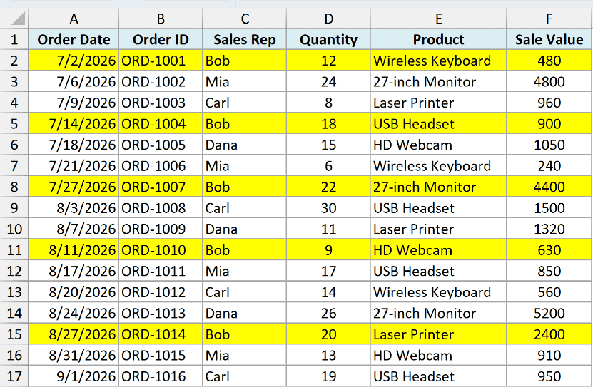
The fix is to write the rule as a formula and lock the column reference. Below I have a dataset where every row with Bob as the sales rep is highlighted.
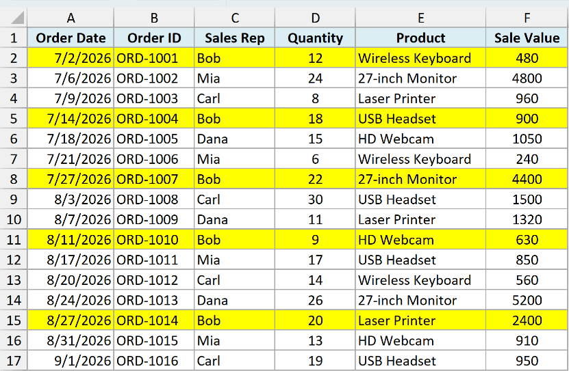
In this article, I’ll show you how to highlight rows based on text, numbers, dates, multiple conditions, a checkbox, and a drop-down selection.
Follow along with the example file
Highlight Rows Based on Cell Value.xlsx
Highlight an Entire Row Based on a Text Value
Let’s start with the most common case, which is highlighting a row when a cell in it contains a specific name.
Below I have an orders dataset, and I want to highlight every row where the sales rep is Bob.
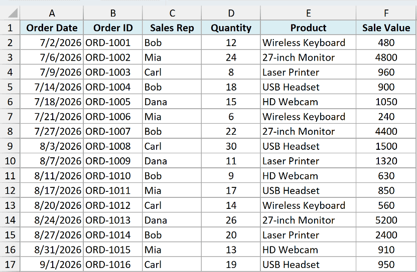
Here are the steps to highlight the rows:
- Select the entire dataset (A2:F17 in this example), but not the header row.
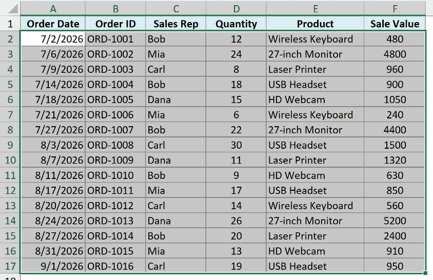
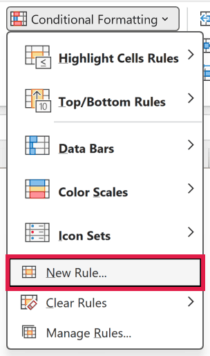
- On the Home tab, in the Styles group, click Conditional Formatting, then click New Rule.
- In the New Formatting Rule dialog box, click ‘Use a formula to determine which cells to format’.
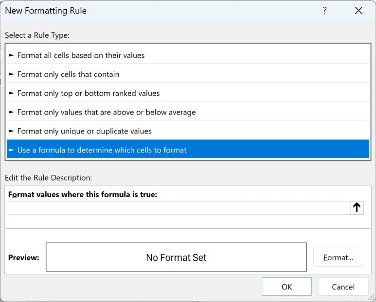
- In the formula field, enter the formula
=$C2="Bob"
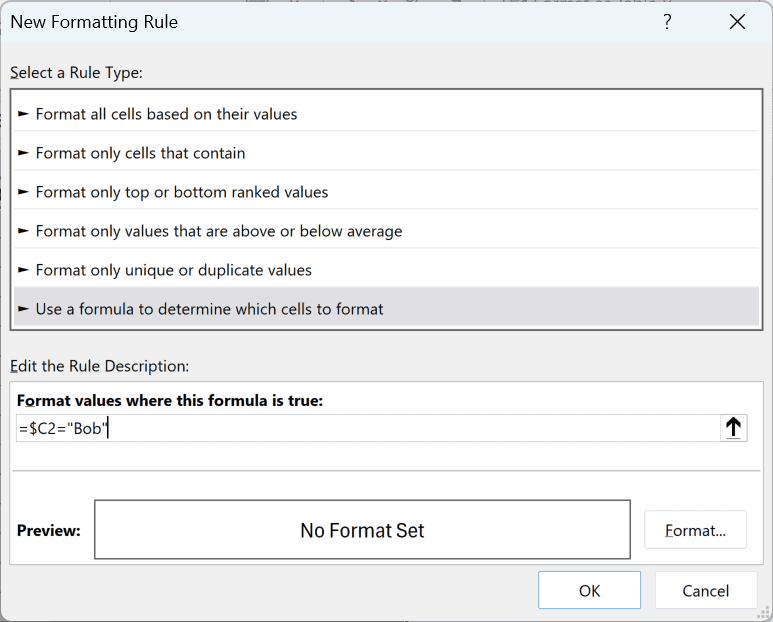
- Click the Format button, go to the Fill tab, and pick the color you want the row highlighted in.
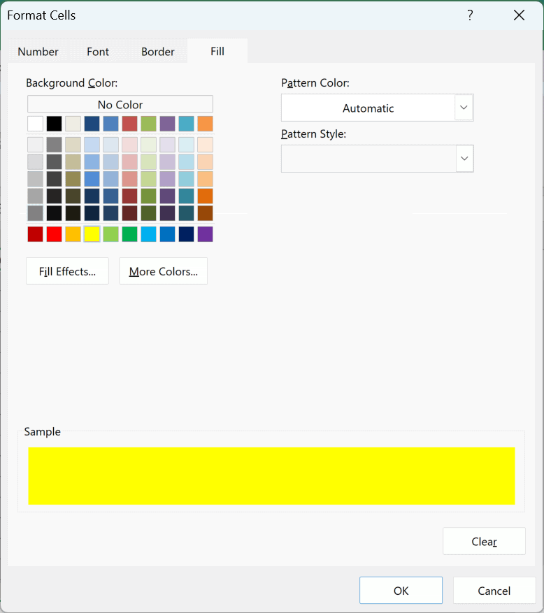
- Click OK, and then click OK again.
Every row where the sales rep is Bob is now highlighted.
How does it work?
Conditional Formatting runs the formula once for every cell in the range you selected, and colors the cell whenever the result is TRUE.
The whole trick is the dollar sign in =$C2="Bob". It locks the column to C, so every cell in a row looks at the sales rep name in that same row.
So when Excel checks cell A2, it reads C2. When it checks F2, it still reads C2. All six cells in row 2 get the same answer, which is why the entire row is colored.
The row number has no dollar sign, so it moves down as Excel works through the range. Cells in row 3 read C3, cells in row 4 read C4, and so on.
Related: Absolute, Relative, and Mixed references in Excel.
The same locked-column trick is what drives conditional formatting based on another column, and it works the same way when you want the rule to read a value in another cell.
Why Only One Cell Gets Highlighted (and How to Fix It)
This is the single most common thing that goes wrong, so it’s worth covering before we get to the other criteria.
You write the rule, click OK, and only the sales rep column turns yellow. The rest of the row stays plain.
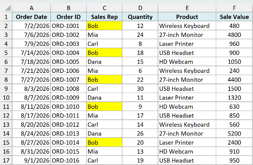
There are only two things that cause this, and both are easy to check.
The rule is applied to one column instead of the whole range. If you had only column C selected when you created the rule, Excel will only ever format column C. That’s the case in the screenshot above.
The column reference isn’t locked. If you entered =C2="Bob" instead of =$C2="Bob", the reference slides sideways as Excel works across the row.
Cell A2 checks C2, but cell B2 checks D2 and cell C2 checks E2.
That second one is worth knowing because of how odd it looks. Only column A gets colored, since A2 is the one cell whose formula still points at the name.
Here is how to repair a rule you have already created, without deleting it:
- On the Home tab, click Conditional Formatting, then click Manage Rules.
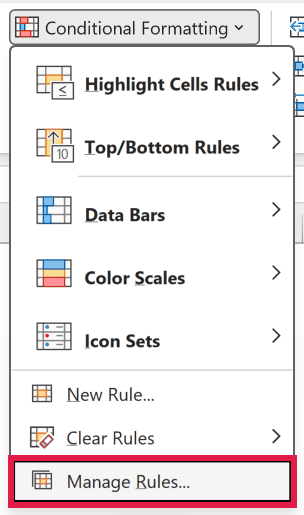
- If your rule isn’t listed, switch ‘Show formatting rules for’ to This Worksheet.
- In the ‘Applies to’ box for your rule, change the range to cover every column you want colored (A2:F17 here), then click Apply.
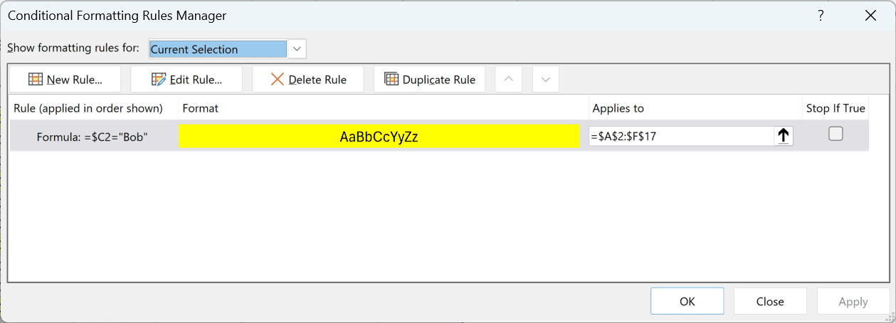
The rule now covers the full width of the data, and the whole row gets highlighted.
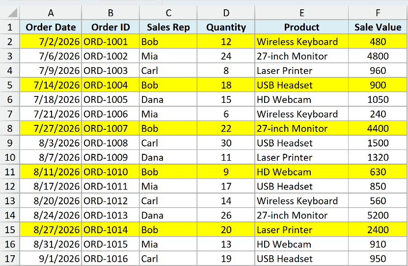
Starting ‘Applies to’ at A1 but writing =$C2 highlights the wrong rows.
Pro Tip: Always write the formula for the top-left cell of the ‘Applies to’ range. If your range starts at row 2, write the formula for row 2.
If your rule is misbehaving in some other way, I have a separate guide on Conditional Formatting not working that covers the rest of the causes.
Highlight Rows Where a Cell Contains Specific Text
The formula we used so far is an exact match. =$C2="Bob" is TRUE only when the cell holds exactly Bob and nothing else.
Quite often you want a partial match instead, where the cell contains the text somewhere inside a longer entry.
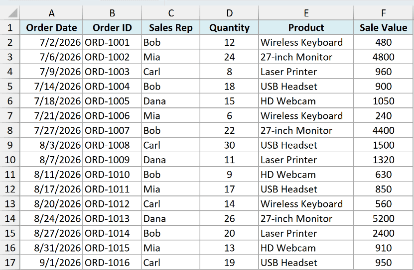
Below is the same dataset, and this time I want to highlight every row where the product is a monitor. The product names are things like ’27-inch Monitor’, so an exact match won’t find them.
Here is the formula to use:
=ISNUMBER(SEARCH("monitor",$E2))
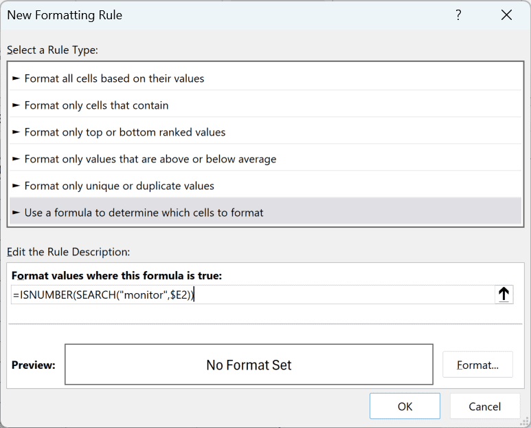
The SEARCH function looks for “monitor” inside the product name and returns the position where it found it.
When the text isn’t there at all, it returns an error instead.
The ISNUMBER function then turns that result into the TRUE or FALSE that Conditional Formatting needs.
A position is a number, so a match gives TRUE. The error from a missing match gives FALSE.
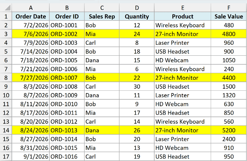
Pro Tip: The SEARCH function ignores case, so “monitor” also matches “Monitor”. For a case-sensitive match, replace it with the FIND function and keep everything else the same.
Highlight Rows Based on a Number Criteria
The same approach works for numbers. You only change what the formula compares.
Below is the same orders dataset, and I want to highlight every row where the quantity is more than 15.
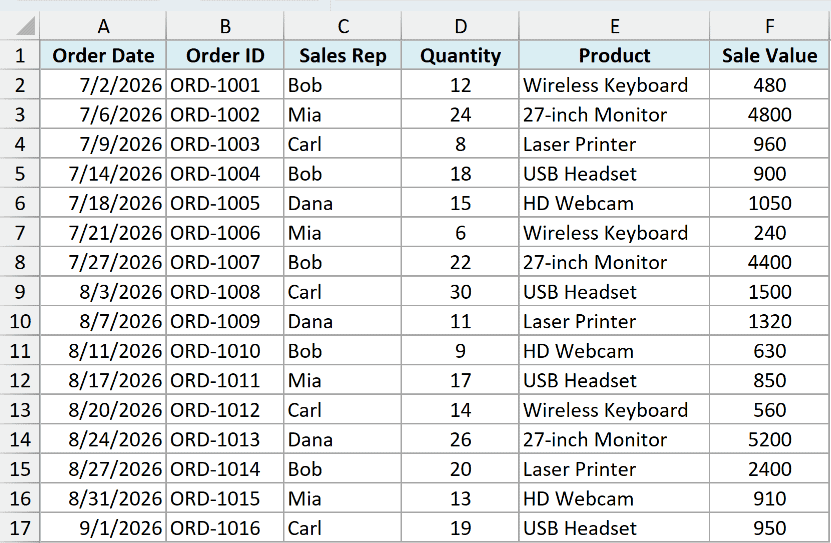
Select A2:F17, go to Home, Conditional Formatting, New Rule, and choose ‘Use a formula to determine which cells to format’. Then enter this formula:
=$D2>15
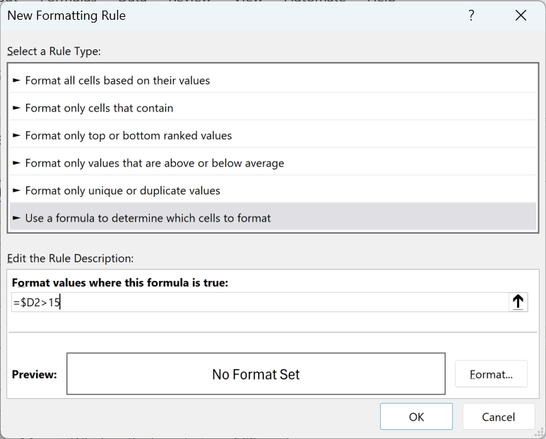
Column D holds the quantity, and the dollar sign locks it the same way it did for the name. Set a fill color, click OK, and every row with a quantity above 15 is highlighted.
If you also want to catch rows where the quantity is exactly 15, use =$D2>=15 instead.
Highlight rows based on a date
Dates are just numbers in Excel, so a date criteria works the same way.
To highlight every row where the order date is after 15 August 2026, use this formula:
=$A2>DATE(2026,8,15)
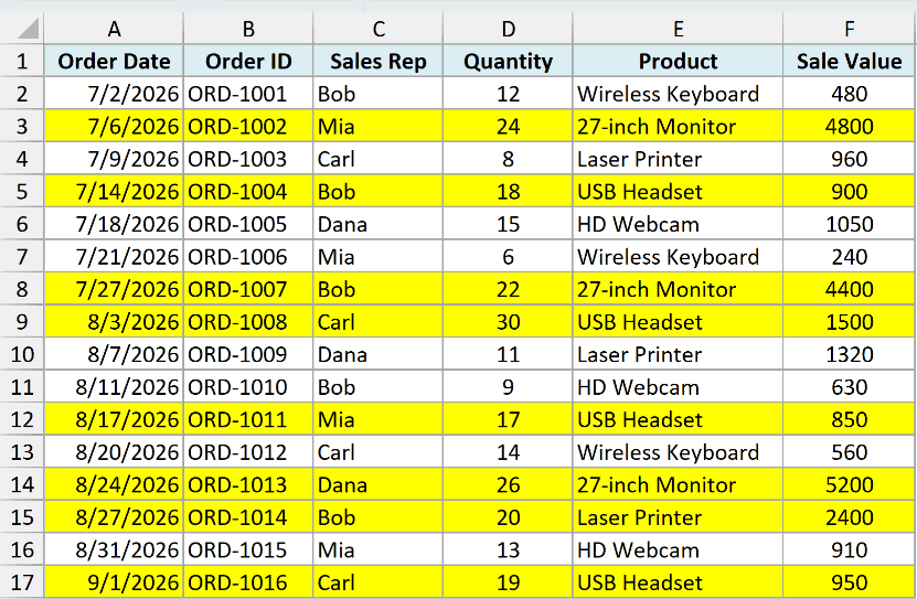
The DATE function builds the cutoff date from the year, month, and day, which is safer than typing a date into the formula and hoping Excel reads it the way you meant.
For deadline and overdue tracking specifically, I have a separate guide on highlighting dates before today.
Pro Tip: For a rolling window that updates whenever you open the file, use the TODAY function. =$A2>=TODAY()-30 highlights rows from the last 30 days.
Follow along with the example file
Highlight Rows Based on Cell Value.xlsx
Highlight Rows Based on Multiple Criteria (AND/OR)
You can also check more than one condition before a row gets highlighted.
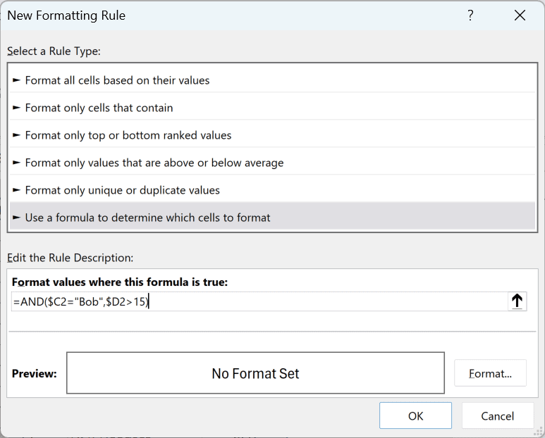
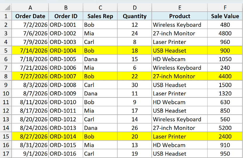
Below is the same dataset, and this time I want to highlight rows only where the sales rep is Bob and the quantity is more than 15.
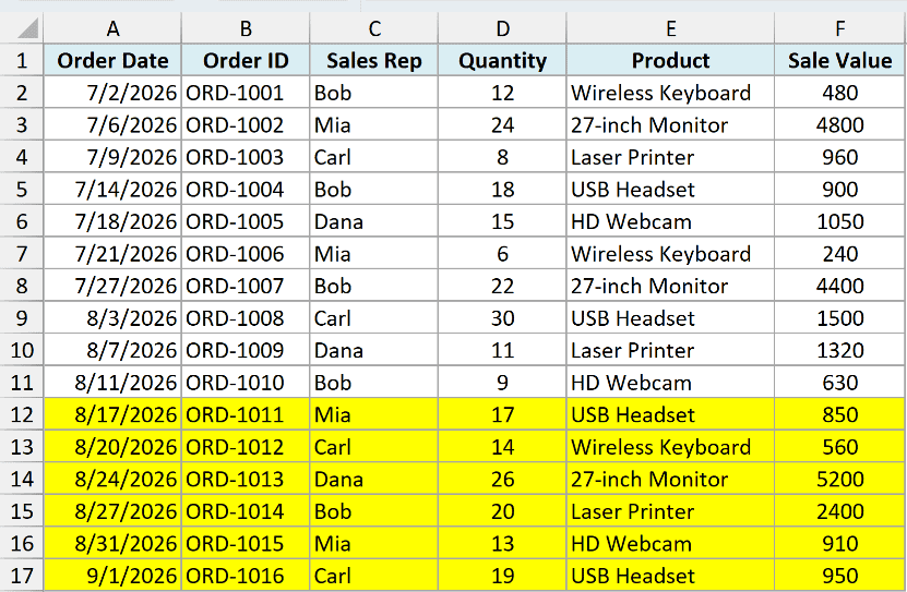
Create the rule the same way as before, and use this formula:
=AND($C2="Bob",$D2>15)
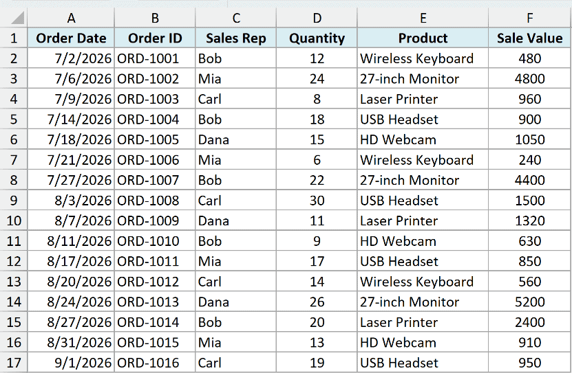
The AND function returns TRUE only when both conditions are met, so Bob’s smaller orders stay unhighlighted.
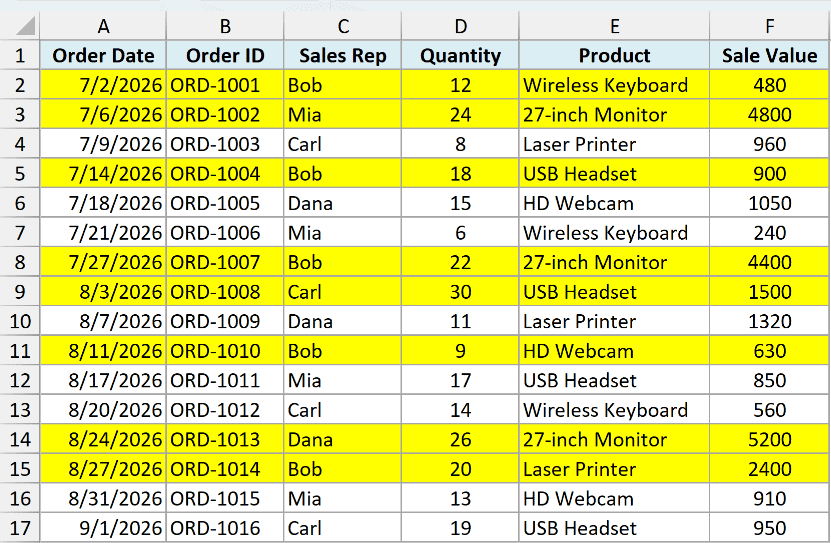
If you want either condition to be enough, use the OR function instead. This formula highlights a row when the sales rep is Bob or the quantity is more than 20:
=OR($C2="Bob",$D2>20)
Both functions take more than two conditions, so you can keep adding checks separated by commas.
Highlight Rows in Different Colors Based on Multiple Conditions
Sometimes one color isn’t enough and you want the rows banded by size.
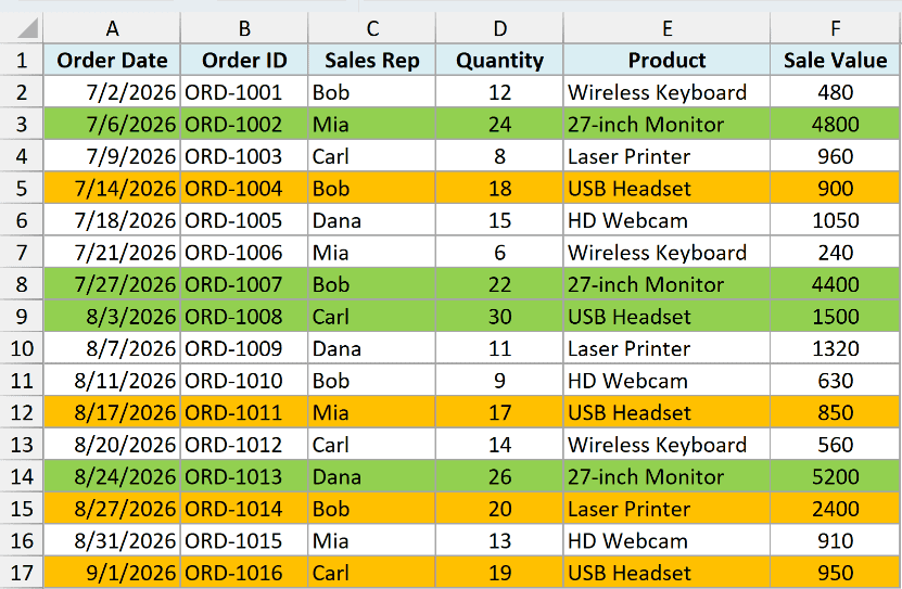
Below is the same dataset, and I want quantities above 20 in green, and quantities above 15 but not above 20 in orange.
This needs two rules, and the order they sit in matters. Start with the orange one:
- Select A2:F17, then go to Home, Conditional Formatting, New Rule, and choose ‘Use a formula to determine which cells to format’.
- Enter the formula
=$D2>15, click Format, set the fill to orange, and click OK twice.
- With the data still selected, open Conditional Formatting again and click New Rule, then enter the formula
=$D2>20and set the fill to green.
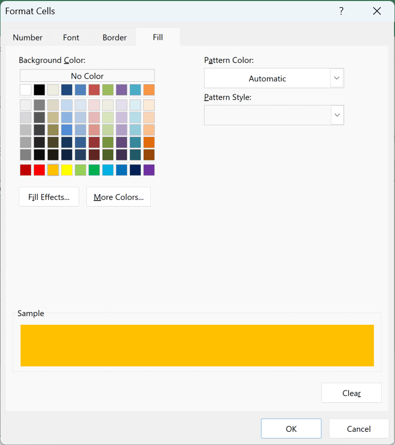
- Open Conditional Formatting, click Manage Rules, and make sure the green rule sits above the orange one. Use the Move Up and Move Down arrows if it doesn’t.
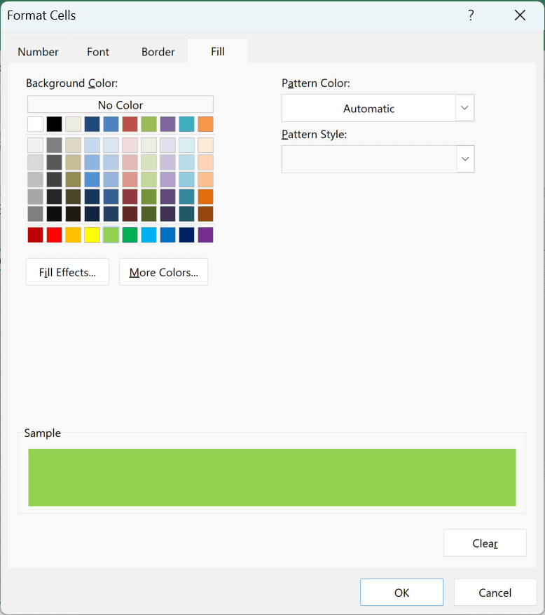
Rows above 20 are now green, and rows between 16 and 20 are orange.
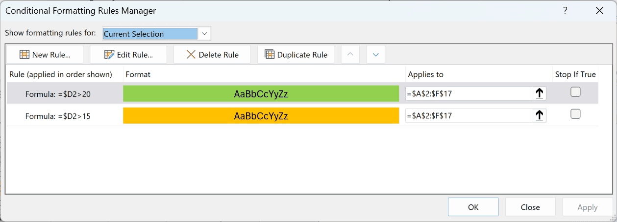
Why the order matters
A quantity of 24 satisfies both rules. It’s above 15 and it’s also above 20.
When two rules want to set the same thing, which is the fill color here, the rule higher up the list wins.
So with green on top, a quantity of 24 comes out green. Flip the order and every qualifying row turns orange, because the =$D2>15 rule is now the one deciding the color for all of them.
Highlight Rows Where Any Cell is Blank
If you’re checking a dataset for gaps, you can highlight any row that has an empty cell in it.
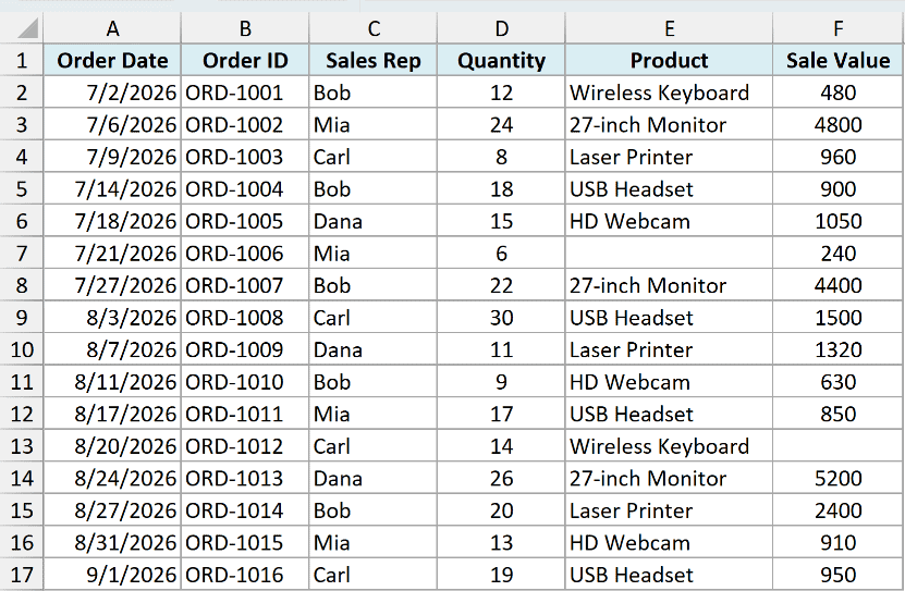
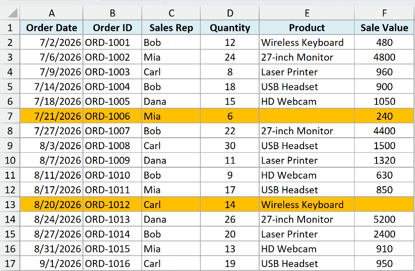
Below is the same dataset with a couple of entries missing, and I want those rows flagged.
Create the rule the same way, and use this formula:
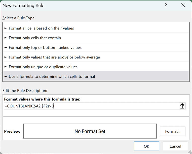
=COUNTBLANK($A2:$F2)>0
The COUNTBLANK function counts the empty cells in that row. If the count is more than 0, there’s a gap somewhere and the row gets highlighted.
Note that both the column letters are locked here, but the row numbers are not. That keeps the formula looking at the full width of the row it’s currently checking.
To do the opposite and highlight only the complete rows, change the comparison to =COUNTBLANK($A2:$F2)=0.
And if you only care about one column being filled in, point the formula at that column instead. =$F2<>"" highlights every row that has a sale value.
Related: read this tutorial if you only want to highlight the blank cells rather than the whole row.
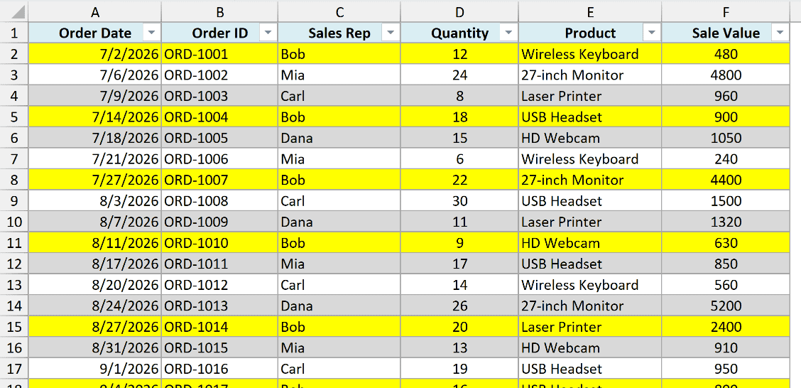
Highlight Rows in an Excel Table (So New Rows Are Covered Too)
There’s one annoying thing about everything we’ve done so far. The rule covers A2:F17 and nothing else, so a row you add underneath doesn’t get highlighted.
Converting the data into an Excel Table fixes that. The rule grows with the table.
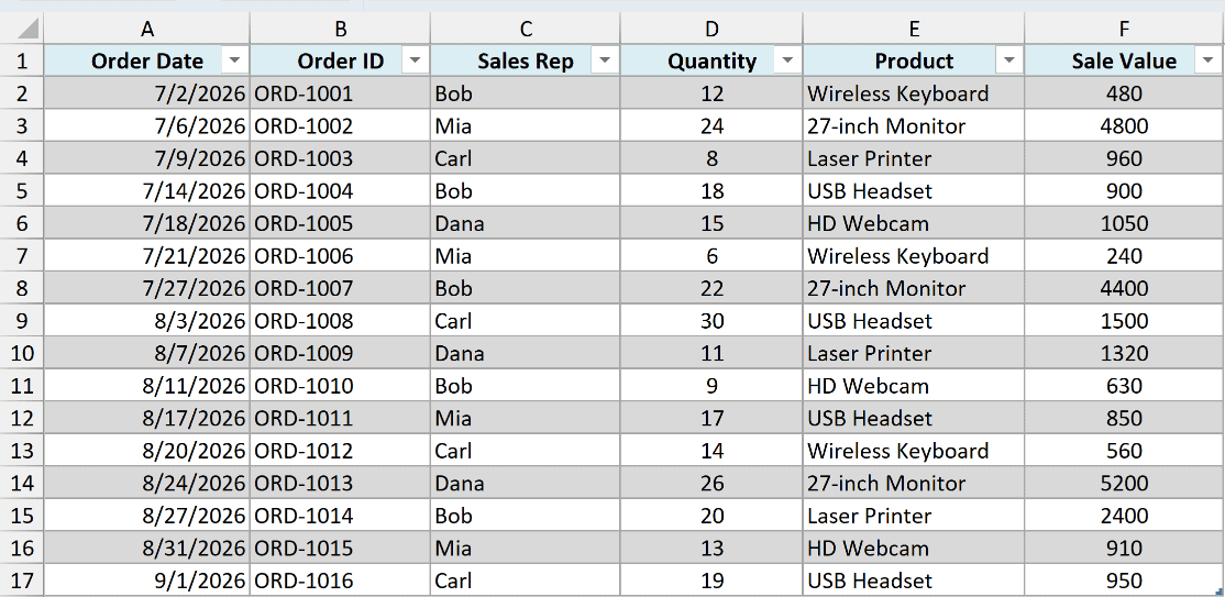
Below is the same dataset, converted into a table by selecting it and pressing Control + T. Here is the full guide on how to create an Excel table.
Now select the table’s data rows and create the rule exactly as before:
=$C2="Bob"
Set your fill color and click OK. The rows with Bob get highlighted, which is what we’d expect.
The useful part happens next. Type a new order in the row below the table, and the table expands to include it.
The Conditional Formatting rule expands with it, so a new Bob row is colored the moment you enter the name.
Pro Tip: Excel rejects the structured reference [@[Sales Rep]] in Conditional Formatting, though it works in worksheet formulas. Use a normal reference like =$C2 here.
Highlight a Row When a Checkbox is Checked
If you’re keeping a task list or an order tracker, a checkbox is a nicer way to mark a row than typing Yes or No.
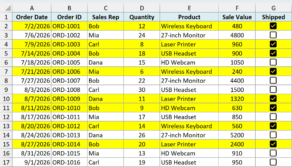
Excel now has real in-cell checkboxes, and because a checked box is simply the value TRUE, Conditional Formatting can read it like any other cell.
Below is the same dataset with a Shipped column in G, and I want the whole row highlighted once an order is marked as shipped.
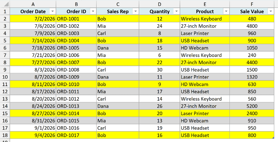
Here are the steps:
- Select G2:G17, then on the Insert tab, in the Controls group, click Checkbox.
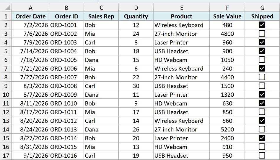
- Select A2:G17, then go to Home, Conditional Formatting, New Rule, and choose ‘Use a formula to determine which cells to format’.
- Enter the formula
=$G2=TRUE, set a fill color, and click OK twice.
Now ticking a box highlights that row straight away, and unticking it clears the color.

In-cell checkboxes are available in Excel for Microsoft 365 on Windows and Mac.
On older versions you would need a Form Control checkbox linked to a cell, and I cover that in my guide on how to insert and use a checkbox in Excel.
Highlight Rows Based on a Drop-Down Selection
In every method so far, the condition has been typed into the rule itself. Changing it means opening the dialog box again.
You can make it interactive instead, so you pick a name from a drop-down and the matching rows light up.
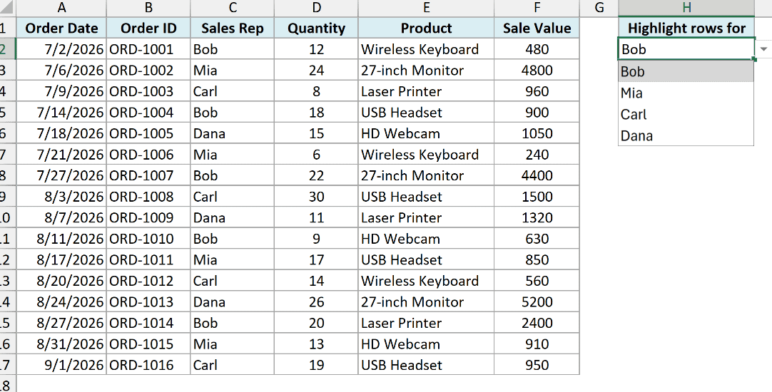
Below is the same dataset with a drop-down in cell H2, and the rows update as soon as I choose a different name.
Here are the steps:
- Create a drop-down list in cell H2 with the sales rep names. Here is a detailed guide on how to create a drop-down list in Excel.
- Select A2:F17, then go to Home, Conditional Formatting, New Rule, and choose ‘Use a formula to determine which cells to format’.
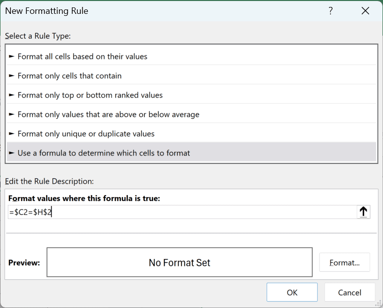
- Enter the formula
=$C2=$H$2, set a fill color, and click OK twice.
Pick any name from the drop-down and the matching rows are highlighted right away.
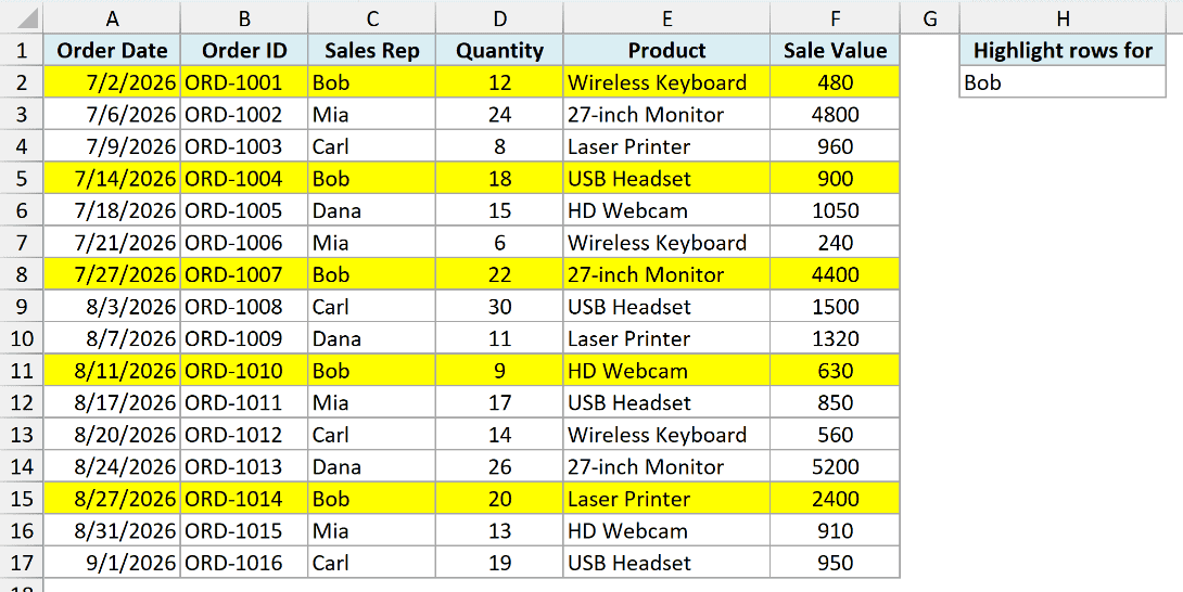
The drop-down cell is the only reference that’s fully locked with =$H$2. Every cell in the data needs to look at that one cell, so both the column and the row are pinned.
If the list of names is long, you can build a drop-down list with search suggestions and the rule will keep working the same way.
Quick Reference: Which Formula to Use
Here is every formula from this article in one place.
In each case, create the rule with ‘Use a formula to determine which cells to format’, and make sure ‘Applies to’ covers the full width of your data.
| What you want to highlight | Formula |
|---|---|
| Rows where a cell equals specific text | =$C2="Bob" |
| Rows where a cell contains text anywhere in it | =ISNUMBER(SEARCH("monitor",$E2)) |
| Rows above a number | =$D2>15 |
| Rows after a date | =$A2>DATE(2026,8,15) |
| Rows from the last 30 days | =$A2>=TODAY()-30 |
| Rows meeting two conditions | =AND($C2="Bob",$D2>15) |
| Rows meeting either condition | =OR($C2="Bob",$D2>20) |
| Rows with any empty cell | =COUNTBLANK($A2:$F2)>0 |
| Rows with no empty cells | =COUNTBLANK($A2:$F2)=0 |
| Rows where a checkbox is ticked | =$G2=TRUE |
| Rows matching a drop-down selection | =$C2=$H$2 |
Things to Keep in Mind
A few things that will save you some time when you’re setting these up.
Write the formula for the first row of your data. If your data starts in row 2, the formula uses row 2. If it starts in row 5, use row 5. Getting this wrong shifts every highlight up or down.
Don’t include the header row in the selection. Headers are text, so a rule like =$D2>15 will treat them oddly and can color the header along with the data.
Conditional Formatting sits on top of manual fill colors. It doesn’t erase them. If a row looks wrong, check whether someone applied a fill color by hand underneath the rule.
Copying cells copies the rules too. Pasting a highlighted row somewhere else brings the rule with it. If that is what you want, here is how to copy conditional formatting to another cell on purpose.
Text comparisons ignore case. =$C2="Bob" also matches “bob” and “BOB”. To make it case sensitive, use =EXACT($C2,"Bob") instead.
You can act on the highlighted rows. Once the colors are on, you can sort by color to group them together.
If the highlight was a shortlist for removal, you can delete rows based on the cell value.
To start over, clear the rules rather than the fill. Clearing the fill color does nothing to a conditional format. Here is how to remove conditional formatting in Excel.
If you want to color alternate rows rather than rows matching a value, that’s plain banding and it needs a different formula. I cover it in Highlight Every Other Row in Excel.
If you want to highlight the row you’re currently clicked in rather than rows matching a value, that’s a different job again, and I cover it in Highlight Active Row/Column in a Data Range.
Interested in learning more on how to search and highlight in Excel? Check the below videos.
These are the ways I use to highlight rows based on a cell value in Excel. I hope you found this article helpful.
Other Excel Articles You May Also Like:
- Apply Conditional Formatting in a Pivot Table in Excel
- Highlight Cells with Formulas in Excel
- How to Create a Heat Map in Excel
- Dynamic Excel Filter, Extracts Data as you Type
- Select Visible Cells in Excel
- How to Delete Every Other Row in Excel
- Excel Table vs Range: When to Use Each
- ISBLANK in Excel

Kind of worked. Selected rows, used basic format of your rule “=$C2=”Bob”. However it highlighted the row above the first instance of “Bob” and didn’t highlight the last instance of “Bob”.
I need help! example…I need a format which shows if any cells in the whole of row 2 say YES (could be more than 1) then I need a visual highlighted cell at the start of that row to flag and tell me I need to look through row 2 (because there a yes along there somewhere).
Thank you so much . Helped a lot
Hey Sumit, great stuff
I followed the first one highlight based on a text value it almost worked but it’s highlighting the row above the one which has the text value in. No idea what I did wrong.
I had the same issue use =$C1=”bob” worked for me
Thanks, excellent – it works very well and it gives a great advantage in displaying dynamic data
Doesnt work. No matter what I try, it doesnt work.
Hello,
My Formatting only seems to work for the first 3 rows, I have tried everything.
Other spreadsheets where I have used this formula work just fine.
Would anyone know what the issue may be?
I select the table, new rule and add: =$b6=”APPROVED”
2 out of 18 work, the rest remain white.
Thank you for explaining WHY the formula does what it does. Understanding why cells behave the way they do is so key to remembering how to make them do it!
If I have a row of 5 cells containing numbers, how can I format it to show where more than one of the cells are greater than zero? the cell content is dynamic!
It works perfectly on a local excel file but stops working when that is uploaded on SharePoint. Any idea how to fix it?
Im trying to apply this rule on a drop down list, to color the entire row based on the options in the list “in process – on hold…” however its not working when typing the text between ” ” i get an error. any suggestions please?
How can i highlight a certain number of rows and columns in a range based on user input? For instance i have a 10×10 range and the user inputs “3” for rows and “5” for columns. How can i turn the cells in the first 3 rows and 5 columns in my range yellow.
How can we adjust this VBA code to only format the data from the active row that is currently selected?
Simple but really usefull. Thanks !
This helped me big time with my 28,000 cell spreadsheet I’m working with. Thank you!!!
Is there a way to highlight a whole row if /any/ value is entered into a cell? For instance: I have a column of “Rejection Reasons” there are any number of different reasons for rejecting a thing (too many for a drop down list), but I want to highlight the row if the thing was rejected for any reason. Can I do that? Basically the opposite of highlighting based on a blank cell.
I think you’d just highlight cells that are greater than zero.
How do I do highlight the entire row directly based on the value I select from the drop-down menu? E.G. not having a SEPARATE drop-down menu: this example, make the cells in the “Sales Rep” column drop downs.
Wouldn’t you just highlight based on specific text? Above, the goal of highlighting based on a drop down selection is to show the rows that contain that text. It sounds like you just want different colors for different Sales Reps, which you could do by using the first tutorial provided here (highlight specific text) where each Rep has their own color.
I got the conditional formatting to work for my pivot. However when any changes are made to the data displayed (e.g., collapsing a row expansion) all the CF rules are reset to apply to the first row in the PT. I using $A$10:$M$308 for the range of the CF; should I somehow do this differently?
I am having a problem using Conditional formatting to find cells with unique values. I have 3 columns across my spreadsheet (D, E & F). I want to compare the 3 values in every row separately. Conditional formatting works great, 1 row at a time. How can I copy the formula down my entire spreadsheet?
I have a problem with this. When I follow the instructions, the whole table is highlighted, but not only one row. What am I doing wrong?
You’re probably missing the dollar sign in front of the column letter. E.e. C3 vs $C3
I followed your instructions and it worked for =$F2=”N/A” Then, I tried adding another formula for a new word =$F2=”PENDING” and it didn’t work anymore. What is the best way to resolve my issue? Thanks in advance
The only thing I can think of is to double check what the formula applies to. If all your data is from A2 down and across to M67, go into the Conditional Formatting drop down, select Manage Rules …, and ensure the Applies to column next to your formulas lists =$A$2:$M$67 so that the formula covers your whole table.
Thanks!!
Wow!! great tutorial. I knew conditional formatting but did not know that one could do so much. Thanks!!
I was actually looking to find out how to highlight a cell based on if a number was greater then or equal to a number in the same row, not a static number, and if it was lower than a number in the same row. I was able to use your formulas here to discover it. If anyone else needs this, I selected my area I wanted to become highlighted, drop down conditional formatting, manage rules, new rule, went to use a formula to determine which cells to format, and then used the following formulas for each rule:
=$E2=$C2
This will cause the formula to look at the two corresponding numbers, so for me, if the generated number is greater than the estimated number, it’s green. Lower than the estimated number, it’s red. Hope this helps someone else out there.
Apparently it didn’t format it properly, the formulas are
=$E2[LESS THAN]$C2
=$E2[GREATER THAN]=$C2
Hopefully this will show up.
Need to know how to highlight a row when the first a cell in column A contains a specific word (not =). What if Bob Dylan? Need whole row highlighted when the cell contains “Bob” regardless of last name or other words contained w/in the same cell.
Ruth, try putting “*Bob*” for the input instead. If anything comes before or after Bob it will be highlighted, so it could be Bob Dylan or Dylan, Bob or Dylan, Bob J. and it will highlight.
I have a column which formats the cell to R/A/G based on priority, how can I also apply another format to make the whole line grey when it is complete, this would be a separate column.
Create a conditional formatting rule for complete and make sure it is listed ABOVE your priority filter in the list of conditional formats applied to that area.
Great tutorial I have always had trouble getting Conditional Formatting to work and it work first time using your tutorial. Don’t know why others say it doesn’t work.
Fantastic
It should be $D1, $D2 highlights the next row instead. Also you need to say that is applies to all the sheet
Really useful. Appreciate it.
How can you do this if you want a row to turn a certain color as soon as on cell is populated? In my case it is populated by a date.
$D2>0 will highlight anything that is not blank.
This did not work for me either. I had to do a workaround to have it come out the way I wanted.
Is there a way to do the first method, but as you go?
Basically a way that you can automatically have the row fill based on one cell, but not have to do the format every time and have this happen as you fill in your spread sheet?
Once you create the rule, you have to change the area it applies to so that it covers your entire table. In the “Conditional Formatting Rules Manager” you’ll select the applicable area for that rule under “Applies to”.
only highlights the cells containing criteria but not the entire row
Once you create the rule, you have to change the area it applies to so that it covers your entire table. In the “Conditional Formatting Rules Manager” you’ll select the applicable area for that rule under “Applies to”.
doesn’t work. tried the first example and it highlighted the row ABOVE where the selected text appeared.
Make sure the D2 is highlighted when you’re creating a rule based on D2.
I had the same issue. When I changed the formula to $C1 instead of $C2 it highlighted the correct row.
you forgot to include the “Applies to” cell range to get it to highlight the full row.
This did not work as I wanted to shade rows where the content was in a ‘Day column to shade rows with ‘Friday’ in them, but the cell was derived by a formula ‘=WEEKDAY(A6)’ so it doesn’t recognise the cell is a Friday
Thanks. Useful information.
It did not work. I have a table(which I then changed back to a range) from A2 to L371. My formula was =L$13=”Inactive”. Column L has blank cells, cells with the word Active, and cells with the word “Inactive”. This method, highlighted mostly cells that said Active, ?? I then capitalized all the INACTIVE rows – still nothing. I’m so confused. Why this didn’t work – does the reference cell need to be the in the beginning?
You put the dollar sign on the row number instead of the column number which means it will only look at the 13th row when evaluating the formatting.
Thank youuu!!!!!
looking for highlight the cells and values belongs to a formula cell
great
hi, If i type the number 5 in excel cell, 5 rows should be need to highlighted in excel . how to do this?
this formula has 2 typos: the quotation marks are closing quotations. Delete these in this formula and replace them and type fresh quotations around the text “Bob”
Highlight Rows Based on a Text Criteria not working for whole row & Also not automatically applies to whole table…
I agree Kristin P, something doesn’t seem right with the explanation for formatting based on text
Is there a typo in the first explanation (Highlight based on Text) as to which cells you select the formula to apply to?
No, it works super fine for me
Thank You Very Very Much…
Your program is contributing to my Excel Growth